프로그래밍 언어 Mini-HOWTO

원저자 : Risto Varanka

원 본 : LDP - Programming Languages HOWTO

번역자 : 주용석 ysjoo@lgeds.lg.co.kr (LG-EDS 공공 1 사업부)

번역일 : 2000년 02월 07일


Index

1. Introduction

2. Programming Languages

3. GUI Toolkits

4. 결론


1. Introduction

Linux는 어떤 유저라도 그것의 개발작업에 참여할 수 있다는 점에서 매우 매력적인 운영 체제 이다. 그러나 언어적인 다양성(The variety of available Program Languages)의 문제는 초기 Linux 개발자들에게 혼동을 주었다. 이 문서는 오늘날의 개발에 있어서 가장 일반적인 옵션들을 listing하였고, 그것들에 대한 핵심적인 사실을 서술한다. 나의 목표는 프로그램 언 어를 review하는 것도 아니고 그 중에 최고를 골라내는 것도 또한 아니다. 각각의 프로그래 밍 언어들은 이용자에게 있어서, 그들이 어떤 일을 하며, 그들의 성향이 어떠한가에 따라 적합화 될 수 있는 하나의 툴이다. 당신이 당신의 귀를 항상 열어놓고, 주위에 자문을 구한 다면, 당신은 보다 많은 정보를 쉽게 얻을 수 있다. 이 글의 Link 섹션은 당신에게 당신 자 신의 연구를 위한 어떤 지침들(some pointers)을 제공할 것이다.

이 문서는 최근에 LDP에 최근에 올라온 것으로 많은 사람들에게 feedback을 받을 기회가 거의 없었다. 그러나 이 글이 Linux상에서 프로그래밍을 하는 것에 관심이 있는 사람에게 유용할 것이라고 입증 될 것을 믿고, 그러한 희망 속에서 배포되었다.

1.1 Copy Right Copyright (c) 2000 Risto Varanka.

1.2 기타

이 문서 역시 다른 LDP문서와 마찬가지로 License에 관한 범위와 Disclaimer와 같은 내용들을 지니고 있으나, 다른 문서들과 동일하게 적용되고 있다.


2. Programming Languages

2.1 Concepts in the Table

Language 일반적으로 일컬어지는 '프로그램 언어'

Beginner 프로그래밍 경험이 거의 없는 사람들에게 쉽게 익숙해질 수 있는지에 대한 여부. "yes"라고 표기된 언어는 초보자에게도 쉽게 습득될 수 있는 언어이다.

Performance '당신이 당신의 응용프로그램을 사용목적으로 만들었을 때, 얼마나 빠르게 이 프로그램이 실행되어지는가'에 대한 척도가 된다. 프로그래밍 언어의 특성보다는 자신의 프로그래밍 알 고리즘 기술에 보다 더 좌우된다. 경험적으로, C, C++, Fortran들은 다른 프로그래밍 언어에 비하여 - 때때로 위의 언어들은 원하는 바를 이루는 것이 어려울지 모르지만 - 우수한 성 능(속도, 메모리) 때문에 이용될 필요성이 제기된다. (언어에 대한 benchmarking을 위한 하 나의 아이디어는 각종의 프로그래밍 언어로 정렬 알고리즘을 구현할 때, 그것들의 속도를 비교해 봄으로써 테스트 해볼 수 있다.) OOP - Object Oriented Programming vs. other paradigms OOP는 많은 대중적인 인기를 얻는 중요한 프로그래밍 패러 다임의 하나이다. 객체지향언 어에 있어서, 자료구조와 알고리즘은 '클래스'라고 불리는 하나의 단위로 통합된다. OOP는 종종 순차적인 프로그램과 대조된다.(자료구조와 알고리즘을 사용하여 대조) OOP라는 방식 은 프로그래밍 언어에 엄격하게 의존되는 것은 아니다. C와 같이 OOP로 간주되지 않는 언 어로도 당신은 OOP로 프로그래밍 할 수 있다. 그리고 OOP로 여겨지는 프로그래밍 언어 로도 순차적 스타일로 프로그래밍 할 수 있는 것이다. 나는 특별한 특성들이나 OOP를 쉽 게 구현할 수 있도록 하는 부가적인 특성을 갖는 OOP언어를 OOP언어로써 listing했다. 기능적인 언어(예를 들자면, Lisp)들은 약간 다른 부류이다 ? 이들 사이에, 기능적 프로그래 밍은 OOP의 superset이다. 그러나 Logic 프로그래밍(Prolog)은 또한 서술적 프로그래밍 (declarative programming)이라고도 불리지만, 이것은 유사한 의미에서 프로그래밍의 다른 유 형과 연관된 것은 아니다.

RAD, Rapid Application Development 당신은 언어를 사용하는데 있어서, 언어자체보다 Tool에 더욱 의존적이다. Linux를 위한 GUI 개발 Tool에 대한 HOWTO가 있으나, 이것은 너무 오래된 것들이다. 당신은 좋은 Graphical Tool을 가지고 RAD를 수행할 수 있다. 뿐만 아니라, 때때로 RAD는 코드 재사용 에 기반을 두므로, Free software들이 좋은 시작지점을 제공할 수 있을 것이다.

Examples 프로그램 언어가 가장 자주 사용되는 영역을 언급한다. 다른 좋은 것(그리고 나쁜 것)은 존재하는 것을 사용한다. 그러나 그것들은 덜 정형적이다.

Comments 수용력이나 Dialects와 같은, 언어상 추가적인 정보


2.2 Major Languages


PERL

Beginner : Yes - OOP : Yes

Examples : Scripting, 시스템 관리, WWW

Comments : 매우 인기 있는 텍스트 및 스트링 제어 툴. 강력한 기능


Python

Beginner : Yes - OOP : Yes

Examples : WWW에 이용되거나 Scripting에 이용. Application 개발가능

Comments :


TCL

Beginner : Yes - OOP : No

Examples : 시스템 관리와 Scripting. Application 개발가능

Comments:


PHP

Beginner : Yes - OOP : Yes

Examples : WWW(WWW server와 연동 되므로 주로 WWW에서만 이용)

Comments : 매우 인기 있는 웹 - 데이터 베이스 연동 언어


Java

Beginner : Yes - OOP : Yes

Examples : Cross platform application(플랫 폼 독립적인 실행), WWW(applet)

Comments :


Lisp

Beginner : Yes - OOP : Functional

Examples : Emacs modes(for elisp)

Comments : Variants Elisp, Clisp and scheme


Fortran

Beginner : No - OOP : No

Examples : 수학적 응용 프로그램

Comments : f77, f90, f95와 같은 여러 버전이 제공


C

Beginner : No - OOP : No

Examples: 시스템 프로그래밍 및 각종 응용 프로그램 개발

Comments : 매우 널리 이용되고 있음


C++

Beginner : No - OOP : Yes

Examples : 응용 프로그램 개발.

Comments :


2.3 Shell Programming

쉘은 역시 가장 중요한 프로그래밍 환경이다. 나는 아직 완전하게 쉘을 이해하지 못했으므 로 그것들을 여기서 다루지 않았다. 원래 Linux 상에서 작업하는 사람을 위해 가장 중요한 것들이 쉘에 관련된 지식이다. 또한 시스템 관리자를 위해서는 이것이 더욱더 필요하다. 쉘 프로그램과 Scripting 언어 사이의 유사점이 있다 - 그것들은 동일한 목포를 이룰 수 있 으며, 그리고 목표를 이루고자 할 때, 당신은 고유 쉘이나 Scripting 언어를 선택할 수 있는 옵션을 가지고 있다. 요즘 가장 인기가 좋은 쉘은 bash, csh, tcsh, ksh, 그리고 zsh이다. 당 신은 쉘들에 대한 정보를 'man'이라는 명령어를 통해 얻을 수 있다.

(역주) 쉘은 유닉스 커널(운영체제)과 유저사이에 명령어를 해석해주는 해석기라고 생각하면 됩니 다. 쉘은 유닉스의 탄생과 더불어 꾸준하게 발전해왔습니다. 처음에는 sh라는 Bourne 쉘을 사용하였으며, BSD유닉스의 탄생과 더불어 Berkeley C shell ? csh가 탄생되었습니다. 그 후 사람들은 Korn 쉘이라는 쉘로써 이 두 쉘을 통합하려는 움직임을 시도했었습니다. 하지만 최근 들어 Bourne Again SHell인 bash와 tcsh이 등장함에 따라 다시 양분화 되고 있습니다. Bourne Again SHell은 이름에서도 보이듯이 Bourne쉘의 특성을 유지한 채 다른 여러 기능 을 보완한 쉘이고 tcsh는 csh의 특징을 유지한 채 다른 기능을 보완한 쉘입니다. 그러니 굳이 sh와 csh를 고집할 필요는 없다고 봅니다. 쉘 스크립터를 통해 여러분은 간단한 프로 그래밍을 할 수 있지만, 사실상 이것은 여러 가지 유닉스의 명령어들의 도움이 없이는 쉽지 않습니다. 쉘은 자체적으로 가지고 있는 명령어들이 많지 않습니다. 다만 컨트롤 제어 및 기타 루프 등을 제공 하고 있긴 합니다.

현재 가장 널리 쓰이는 쉘이 바로 bash인 것 같습니다. 모든 쉘들에는 장단 점들이 있지 만 ksh가 스크립팅 기능이 가장 강력하고요, bash와 tcsh는 프로그래밍 보단 주로 사용자 편의를 위해 많은 기능을 제공 하고 있습니다. 과거 csh에서 볼 수 없었던 command editing기능, 그리고 다양해진 job control 과 강력해진 history기능들이 바로 그것입니다.

제가 아는 것이 짧은 관계로 대충 쉘에 대해선 이정도만 덧붙히려고 합니다. 더 많은 정보 를 원하시면 ysjoo@lgeds.lg.co.kr로 메일 주시기 바랍니다. 참고로 저는 Bourne Again SHell 을 사용하고 있습니다. ;-)


2.4 Other Languages Other languages of note

: AWK, SED, Smalltalk, Eiffel, ADA, Prolog, assembler, Object C, Pascal, Logo


2.5 Other Links

A general info site : http://www.tunes.org/Review/Languages.html

TCL : http://www.scriptics.org

PERL : http://www.perl.org

Python : http://www.python.org

PHP : http://www.php.net

Java : http://www.javasoft.com

clisp : http://clisp.cons.org/~haible/packages-clisp.html


3. GUI ToolKits


3.1 Concepts in the Table

Library 툴 키트의 약자 또는 일반적인 이름을 의미한다.

Beginner 새로운 프로그래머 에게 툴 키트가 배우기 적당한지에 관한 여부

License 다른 GUI툴 키트를 위한 다른 License는 실제적으로 중요성을 가지고 있다. GTK+와 TK License는 당신이 open source와 closed source application 개발에 있어서, 특별한 license 의 대가 없이 제공된다. 그러나 Motif는 모든 개발에 있어서 license에 대한 지불을 요구 하고 있으며, Qt의 경우 closed source형태로 개발되는 일에만 지불을 요구하고 있다.

Language 툴 키트와 함께 가장 자주 이용되는 프로그래밍 언어

Bindings 툴 키트와 함께 사용될 수 있는 다른 프로그래밍 언어

Examples 툴 키트와 프로그래밍 언어로 만들어 질 수 있는 응용 프로그램

Comments 언어와 툴 키트에 관한 추가적인 사항 및 정보


3.2 Major GUI ToolKits


TK

Beginner: Yes - License: Free

Language: TCL Bindings: PERL, Python, C, C++, others

Examples: X window Programming, TKDesk, Make xconfig


GTK+

Beginner: No - License : Free(LGPL)

Language: C Bindings: PERL, C++, Python, many others

Examples: GNOME, Gimp


QT

Beginner: No - License: Free for open source

Language: C++ Bindings: Python, PERL, C, others?

Examples: KDE


Motif

Beginner: No - License: Non-free

Language: C, C++ Bindings: Python, others?

Examples: Netscape, WordPerfect


3.3 Links

TK : http://www.scriptics.com

GTK+ : http://www.gtk.org

QT : http://www.troll.no

Motif : http://www.metrolink.com


4. 결론


원래 이 글에는 결론 부분이 없었습니다. 그러나 위의 설명만으로는 너무나 간략하게 모든 것이 설명된 것 같았고, 더구나 원 저자 또한 이 글이 변경되는 것에 대한 License가 덧붙혀 진 부분에 대한 언급만을 요구 했으므로, 결론을 덧붙혀 보고자 합니다.

먼저 프로그램 언어의 선택 문제입니다. 사실상 프로그래밍 언어의 선택은 완전한 개발자의 문제라고 생각됩니다. 사실상 프로그램의 완성도는 그 프로그램이 얼마나 사용자의 구미에 맞게 작성되었으며, 얼마나 효율적인 알고리즘을 사용했으며, 얼마나 많은 조사와 검증을 거 쳤느냐에 따라 달라지는 것이라고 생각합니다. 하지만 같은 길을 걸어가더라도 지름 길이 있 듯이, 어떤 프로젝트에도 적절한 프로그래밍 수단이 따른다고 생각됩니다. X windows환경에 서 단순히 X-libraries와 C만을 가지고 프로그래밍하는 것은 사실 너무나 많은 부담을 프로 그래머에게 떠넘기는 일입니다. 간단한 응용 프로그램을 위해 그런 어려운 툴 키트를 가지고 프로그램 하는 것 보다는 GTK나 Motif와 같은 편리한 툴 키트를 이용하는 것은 매우 효율 적인 방법이라고 저는 믿습니다. 비록 응용프로그램의 정교성 및 효율성, 수행 속도 측면에 선 다소 뒤질 지 모르지만, 상호 trade-off가 있는 것이겠죠.

이런 프로그램 언어의 선택은 여러 프로그래머의 역할 인 것이죠.

이제 제 경험을 토대로 제가 사용 하였던 프로그램 언어에 대해 설명을 하고 이 글을 마무 리 짓겠습니다.

자바라는 언어는 1995년도에 처음 Sun사에서 선보인 언어 입니다. 사실상 가장 충실한 OOP의 구조를 지니고 있다고 볼 수 있습니다.(완전히 제 개인적인 견해 입니다.) 많은 프로 그램을 짜본 것은 아니지만, 자바의 클래스 개념은 가장 완벽한 것이라고 볼 수 있을 것 같 습니다. 물론 개인적인 차이는 분명히 존재 하겠죠. 하지만 플랫 폼에 독립적이고 비교적 배 우기 쉬우며, Web Based Programming이라는 차원에서는 단연 우위를 자랑한다고 볼 수 있 습니다.

C는 설명할 필요가 없는 언어입니다. 간결한 문법과 강력한 포인터라는 점은 이 C언어의 가장 큰 장점이자 또한 언어 자체에 대한 이해를 어렵게 하는 약점이라고 볼 수 있습니다. 하지만 대부분의 시스템 프로그래밍들이 바로 이 C언어를 기반으로 이루어지고 있고, 아직 까지 많은 운영체제의 개발이 이 언어에 의존하고 있습니다. 정교한 제어와, 빠른 속도, 그리 고 작은 바이너리 사이징은 매우 뛰어난 C언어의 장점입니다. 하지만 OOP를 위한 어떠한 수단도 제공하지 않고 있다는 점에서 구시대적인 프로그래밍 언어라고 간주 되고 있습니다. 이러한 점을 보완하기 위해 새로이 Objective - C라는 컴파일러가 새로 탄생하였습니다. 많 은 컴파일러가 존재 하나 대부분 ANSI - C 표준을 따르고 있습니다. 또한 Linux 시스템 프로 그래밍 표준을 위해 POSIX가 제공되고 있습니다.

C++는 현재 OOP 라는 패러 다임을 구현하는 데 있어서 가장 널리 사용되고 있는 프로그 래밍 언어라고 생각합니다. 또한 Microsoft사의 제품 군들이 모두 MFC라는 강력한 클래스 라이브러리를 제공 하고 있기 때문에 매우 인기 있는 언어입니다. C만큼이나 많은 컴파일러 가 제공되고 있습니다. Linux환경에서는 GNU g++가 가장 일반적인 컴파일러로 이용되고 있 습니다.

저도 스크립트 언어에 대해서는 많은 지식을 갖고 있지 않지만, 흔히 간단한 스크립트를 작 성하기 위해선 shell script와 PERL스크립트를 이용합니다. PERL은 또한 shell스크립트 보 다 훨씬 많은 built-in 명령어를 가지고 있으며, 텍스트 제어에 매우 강력한 기능을 제공합니 다. 또한 풍부한 라이브러리들은 PERL을 스크립트 언어 수준을 뛰어넘을 수 있게 도와줍니 다. 그리고 위 들 스크립트 언어들은 CGI 프로그래밍에서 자주 이용되고 있습니다.

웹 개발환경에서는 새로 등장한 스크립트 언어가 바로 PHP입니다. 강력한 텍스트 제어 기능 뿐만 아니라 웹 서버가 직접 parsing 해서 처리한다는 점이 이 PHP의 장점이기도 합니 다. (속도 측면에서 좀 유리한 것 같더군요) 그리고 CGI 및 동적 웹 환경을 위해 제공되는 많은 라이브러리와, 데이터베이스 별로 제공되는 Interface Set은 매우 강력한 힘을 발휘 할 수 있습니다. 하지만 개인적인 판단으로 보안적인 차원에 문제가 있을 수도 있다고 생각됩니 다.

이밖에도 저는 지금까지 프로그래밍을 해오면서 몇 가지 언어를 더 사용해 보긴 했지만 여기서 언급할 수준이 아니라고 생각합니다. 다른 의문 사항이 있다면, ysjoo@lgeds.lg.co.kr로 메일을 주시면 아는 범위 내에서 성실하게 답변해 드리겠습니다.

Feature: Programming

Open source programming languages for kids

By Ryan McGrath on December 19, 2008 (2:00:00 PM)

The past couple of years have seen an explosion of open source programming languages and utilities that are geared toward children. Many of these efforts are based around the idea that, since the days of BASIC, programming environments have become far too complex for untrained minds to wrap themselves around. Some toolkits aim to create entirely new ways of envisioning and creating projects that appeal to younger minds, such as games and animations, while others aim to recreate the "basic"-ness of BASIC in a modern language and environment.

Scratch

Scratch. Click to enlarge.

Developed by the Lifelong Kindergarten group at MIT, Scratch is a graphical programming environment implemented in Squeak that works in a very Lego-like fashion. The basic premise is that you build programs by snapping together colorful blocks of code. Scratch's custom interface allows a programmer to bring in graphics and sounds and create basic animations. All the basic programming constructs, such as loops and if statements, are supported, and grouped into different block categories, such as Motion, Sensing, and Sound.

Scratch has implementations available under Microsoft Windows and Mac OS X, but as of yet there's no (official) native Linux version to run. It is possible to run Scratch through Wine, though in my tests most audio-related Scratch programs ended up failing. There is a Linux-runnable version of Scratch, though it's not actively developed by the folks at MIT. The one problem with using this version is that presentation mode, where your Scratch program can take over the whole screen, doesn't work. This isn't really a show-stopper, as there are a few different ways to view a Scratch program, but it's easy to see how it could be a desired feature.

One useful prospect that Scratch offers is the ability to upload your programs to the Scratch Web site, where you can create an account, get support, and browse programs that other Scratch users have uploaded. All uploaded programs are open source, in the sense that you can download and modify the source of any Scratch program that's been uploaded. Scratch programs are also viewable from within a Web browser, for the most part, through use of a Java applet called the Scratch Player. Scratch itself is released under its own Scratch License, and all uploaded programs exist under a Creative Commons Share Alike license.

One issue I came across with Scratch was that the source code for a program could become quite large when the program involved many graphics or, more specifically, music. One program, a simple music player, reached a strikingly large 93MB in size. Typically Scratch would choke on loading any program greater than 60MB in size, usually erroring out. The large size of a file may have something to do with how old the source code is; repeated instances of saving and re-opening the same file seemed to grow the size exponentially.

Alice. Click to enlarge.

Alice

Scratch deals well with 2-D graphics, text, and other somewhat "flat" programming concepts. By contrast, Alice teaches programming fundamentals in the form of 3-D movies and games. Alice is developed in Java, and is somewhat like Scratch in that you build things in a drag and drop interface.

Alice, developed by a group of researchers at Carnegie Mellon University, has releases for Linux, Mac OS X, and Windows, and is released under an aptly titled Alice License. The environment is open source in the sense that you can download and examine the source code, but the creators prefer to work exclusively in-team, and don't take outside contributions. Alice has been around since 1999, making it one of the oldest and most developed environments for teaching children how to program. It is because of this that it's used in schools all over the world.

Shoes

Originally created by a developer who goes by "why the lucky stiff," now furthered by a large development community, and based on the already user-friendly Ruby programming language, Shoes is an open source toolkit that's a bit more in line with traditional programming methods. All that's required to make a program in Shoes, besides its runtime environment, is a basic text editor. On the project's Web site you can find a free PDF guidebook that contains tutorials and examples for Shoes. You can also order the guidebook in paperback form for $5.57. Shoes 2 comes with an extensive built-in manual that users can access via key commands.

Shoes. Click to enlarge.

Shoes has similar syntax to Ruby, and has easy methods for creating graphics and buttons, as well as displaying colors and text. It is supported across multiple platforms, including Linux, Mac OS X, and Windows. The toolkit works well across platforms, in that windows, buttons, and dialogs look native to their environment, and do so regardless of which platform the application was initially created on. A benefit of Shoes being in Ruby is that it's given access to the many different RubyGems packages that exist. Shoes 2 even includes support for automatically installing a Gem on a user's system if it's not already present.

Shoes has a fan-supported Web site that showcases a gallery of applications created with Shoes. As with Scratch, all the applications that are uploaded can be downloaded, modified, and remixed. Shoes itself is released under an MIT License, and is open to outside patching and development.

A multitude of other programming languages and environments exist to teach children, such as Greenfoot, Phogram, and Microsoft's Small Basic, though many of them exist as proprietary implementations. Scratch, Alice, and Shoes are all open source, include support channels such as forums or chatrooms, and have large, thriving communities. These three environments are possibly the most open, mature, and easily accessible environments that are geared toward teaching programming concepts to young minds.

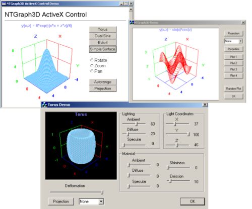
VC++ Example Source: 2D Chart and 3D Plot Print Chart Control

By Kris Jearakul

Environment: Visual C++ 6.0,Win 95/98,NT4.0.
The print routine has been tested with HP Laserjet 4ML and Lexmark 3200, with Acrobat Writer by setting the resolution at 600 dpi.

Introduction

The CChart class is the class derived from CWnd class. The class provides the functionality of Windows plotting chart control . The chart plotted from this class will look like the output of an Oscilloscope . By the way, I found that there is an article like this already posted here . So CChart3d is the derived class from CChart that will be able to plot data in 3D style. The demo project will will plot data in 2D and 3D like a Waterfall plot found in an expensive Signal Analyser.

Implementing

CChart and CChart3d to your project First add these four files to your project. Chart3d.cpp , Chart3d.h , Chart.cpp and Chart.h . Then you can add the object to like this :
CChart m_Chart2d ;CChart3d m_Chart3d;
After that you can customize, create and then update new data to chart respectively. In the demo project you can find the implementation of CChart and CChart3d in the routine
CWFDemoView::InitialUpdate();   // for customizing and creating chartCWFDemoView::OnTimer();         // for updating data to chartCWFDemoView::OnPrint(CDC *pDC); // for printing chart.

Customize Control

Customize control of chart can be done before and after the chart is created. If you change setting after the chart was created then call function Invalidate() to redrawn the chart.
  1. Setting Chart Title can be done by calling the function
    SetChartTitle(Cstring str)
  2. Setting Range of each axis can be done by calling the following functions:
    CChart::SetRange(double Xmin, double Xmax,                 double Ymin, doubleYmax)Default: SetRange(-10,10,-10,10)CChart3d::SetRange3d(double Xmin, double Xmax,                     double Ymin, double Ymax,                     double Zmin , double Zmax)Default: SetRange3d(0,100,0,20,0,100)
  3. Setting the Axiss Label can be done by calling the functions:
    CChart::SetAxisLabel(Cstring strLabelX , Cstring strLabelY)
  4. Setting the number of grid scale for each axis and the labels to be plotted on screen can be done by calling the functions:
    CChart::SetGridNumber(int nGridX , int nGridY)CChart3d::SetGridNumber3D(int nGridX, int nGridY, int nGridZ)
    Note: Grid labels will be automatic drawn according to the number of grid setting.
  5. Setting the Axis style by calling the function:
    CChart::SetAxisStyle(int nStyle)                     //0: Single Quadrant                     //1: Double Quadrant                     //2: 4 Quadrant *default
  6. Customize color on chart Background Color can be modified with variable: m_BGColor. Axis color can be modified with variable: m_AxisColor. Grid color can be modified with variable: m_GridColor. Series plot color can be modified with variable: CSerie::m_plotColor.

    Example

    mChart.m_BGColor = RGB(255,0,0,)               //Set background color to redmChart.m_AxisColor = RGB(0,0,0);               // Set background color to blackmChart.m_GridColor = RGB(120,120,120);         // Set grid color to gray .<mChart.mpSerie[0].m_plotColor = RGB(0,255,0) ; //Set series 0 color to green
  7. Set the number of series on chart by modify variable
    CChart::nSerieCount.

    Note: The maximum series on the code is 60 but you can assemble it and change to any number is your want.

  8. Allocate number of points for all series by calling function:
    CChart::AllocSerie(int nSerie)

    Caution : Setting the number of series has to be done before calling this function

  9. Working with the Chart
    • Creating Chart - After you finished customizing the chart then call the function:
      Create(DWORD dwStyle, CRect &rect, CWnd *pParent, UINT id)

      Example:

      mChart.Create(WS_CHILD|WS_VISIBLE,Rect,this,12000);
    • Updating Chart - You can update data for each series by calling function :
      SetXYValue(double x , double y , int index , int nSerieIdx).

      If you want chart to be redrawn function Invalidate() should be called . The chart background will be drawn as it was when the chart was first created then it will save the background in the buffer. But if you changed background color or grid color then you need to call the Invalidate() function with argument FALSE to force the chart background to be redrawn .

    • Printing Chart - In the demo project you can preview and print the chart . I have test the program with several printers. The function CChart::PrintChart(CDC *pDC,int x ,int y) is used for printing the chart.

      In the demo project I added this function in OnPrint(CDC *pDC) in CFormView class as example :

      void CWFDemoView::OnPrint(CDC* pDC, CPrintInfo* /*pInfo*/){ m_Chart2d.PrintChart(pDC,500,200); m_Chart3d.PrintChart(pDC,500,1800);}

Downloads

Download demo project - 29 Kb
Download source - 10 Kb
Click here to Skip to main content 1244073422_geometry.zip
General Programming » Algorithms & Recipes » Computational Geometry Intermediate License: The Code Project Open License (CPOL)

Classes for computational geometry

By Chris Maunder

Some classes and utility functions for general computational geometry
VC6, VC7Win2K, WinXP, Visual Studio, MFC, Dev
Posted:26 Dec 2001
Views:135,231
Bookmarked:71 times
34 votes for this article.
Popularity: 7.11 Rating: 4.64 out of 5
2 votes, 11.8%
1

2

3

4
15 votes, 88.2%
5

Introduction

This article presents two classes and a set of utility functions for computational geometry. C3Point is a 3D counterpart to CPoint and CPolygon encapsulates a set of C3Point's and provides general polygon handling functions. The classes have been mildly optimised for speed. The classes were originally written for use in discretising 2D surfaces into element networks and for calculating properties of the resultant elements. Care must be taken when using some of the functions such as the curvature and area functions to ensure that the results returned by the functions are consistent with your needs and definitions.

The classes make use of a typedef REAL that is either double or float depending on whether USING_DOUBLE or USING_FLOAT has been defined in geometry.h. Obviously using template classes would have been neater, but these classes were developed to get a job done, not to be the epitome of structured programming. A number of conversion functions have been provided:

D2Real(x) (x)             // double => REALF2Real(x) (x)             // float => REALReal2D(x) (x)             // REAL => doubleReal2F(x) ((float)(x))    // REAL => floatInt2Real(x) ((double)(x)) // int => REALReal2Int(x) ((int)(x))    // REAL => intReal2Int(double d0)       // REAL => int (faster than a (cast)).

All the classes and utility functions are provided 'as-is'. I've been meaning to write this class up for a long time and figured it was best to at least post something than nothing at all.

C3Point

C3Point is a 3D counterpart to CPoint. It contains 3 data members x,y and z and a set of functions for calculating properties, scaling, translating and for arithmetic operations.

class C3Point {// Attributespublic:    REAL x,y,z;//Operationspublic:    C3Point() {}                          // constructor    C3Point(double x, double y, double z) // constructor    REAL Length2()                        // length squared    REAL Length()                         // length    void Scale(REAL factor)               // scale by a factor    void Normalise();                     // convert to a unit length    void operator=(C3Point& P)            // assign    C3Point operator-(C3Point P)          // subtract    C3Point operator-()                   // unary -    C3Point operator+(C3Point P)          // add    C3Point operator+=(C3Point P)         // add +=    C3Point operator-=(C3Point P)         // subtract -=    REAL operator*(C3Point P)             // vector dot product    C3Point operator*(REAL f)             // scalar product    C3Point operator/(REAL f)             // scalar div    C3Point operator*=(REAL f)            // scalar mult *=    C3Point operator/=(REAL f)            // scalar div /=    C3Point operator^(C3Point P)          // cross product    BOOL operator==(C3Point& P);          // is equal to?    BOOL operator!=(C3Point& P)           // is not equal to?};#define VECTOR C3Point

CPolygon

CPolygon encapsulates a set of C3Point's and provides general polygon handling functions.

CPolygon();CPolygon(int);                     // Construct with a preallocated number of 
// points
BOOL Closed(); // Is the polygon closed?int GetSize() // Number of points// is vertex 'index' between start,end inclusive?BOOL InSpan(int start, int end, int index); // is vertex 'index' between start,end exclusive?BOOL InSpanProper(int start, int end, int index); BOOL PointIn(C3Point P); // Is point inside polygon?BOOL SetSize(int); // Change size of polygonvoid RemoveAll() // Empty polygon of all pointsBOOL Trim(int, int); // Trims polygon down so that points before // "Start" and after "End" are removed. // Start and End must be in the range
// 0..GetSize()-1
BOOL Close(); // Make polygon closedBOOL Add(C3Point); // Add point to polygonBOOL SetAt(int nPos, C3Point& p); // set vertex nPos as point pvoid Delete(int); // Delete a vertexBOOL InsertAt(int nPosition, C3Point P); // insert point P at pos nPosition
// (0..N-1)
void FreeExtra(); // Free extra memory left over after
// deletes
int PointSeparation(int Point1, int Point2); // Distance (in pts) between 2
// points
void Rationalise(int nAngle); // Combines adjacent line segments if the
// angle between them is less than nAngle
// (degrees).
REAL SegmentLength(int,int); // Length of a segment of the polygonC3Point GetClosestPoint(C3Point p, int *nIndex = NULL);REAL Area(); // returns polygon areaC3Point Centroid(); // Calculate centroid of polygonBOOL GetAttributes(REAL *pArea, C3Point *pCentroid, C3Point *pNorm, REAL *pSlope, REAL *pAspect);BOOL Diagonal(int i, int j); // Returns TRUE iff (v_i, v_j) is a
// proper internal or external
// diagonal of this polygon
virtual void Translate(VECTOR v); // Translate polygonBOOL Intersected(C3Point& p1, C3Point& p2); // Does p1-p2 intersect
// polygon?
BOOL IntersectedProp(C3Point& p1, C3Point& p2); // Does p1-p2 intersect
// polygon properly?
BOOL Triangulate(CPolygon*); // Triangulate: Ear clip triangulationBOOL CPTriangulate(CPolygon*, C3Point); // Central point triangulationBOOL DelauneyTri(CPolygon*); // Triangulate: Delauney triangulation
// Load polygon from X-Y or X-Y-Z data fileBOOL LoadXY(LPCTSTR Filename, REAL Zdefault = D2Real(0.0));BOOL LoadXY(FILE* fp, REAL Zdefault = D2Real(0.0));BOOL LoadXYZ(LPCTSTR Filename, BOOL bWarn = TRUE);BOOL LoadXYZ(FILE* fp);// Save file either as://    Num Points, elevation, x-y pairs...,// or//    x-y-z triplets...BOOL Save(LPCTSTR Filename, BOOL bAsPoints = FALSE, BOOL bWarn = TRUE);void NaturalSpline(double*& b, double*& c, double*& d); // Natural cubic 
// spline
REAL Curvature(int i); // Curvature at vertex
// i
REAL Curvature(int nIndex, int nSampleSize); // Avg curvature at i
// over a number of
// points
C3Point& operator[](int index);C3Point& Point(int index);void operator=(CPolygon& P);

General Functions

These functions provide general routines for vectors (C3Points) and polygons.

inline REAL Dot(C3Point V1, C3Point V2)       // dot productinline C3Point Cross(C3Point p1, C3Point p2)  // cross product
C3Point GetClosestPoint2D(C3Point& start, C3Point& end, C3Point& P);REAL   Angle(C3Point, C3Point, C3Point);    // Angle between 2 vectors formed 
// from 3 points (deg)
REAL Angle(VECTOR v, VECTOR u); // Angle between 2 vectors
// (degrees)
REAL TriArea2(C3Point, C3Point, C3Point); // Area^2 between 2 vectors formed
// from 3 points
REAL TriArea2(VECTOR u, VECTOR v); // Area^2 between 2 vectorsBOOL IntersectProp(C3Point a, C3Point b, // Returns true iff ab properly C3Point c, C3Point d) // intersects cd: they share
// a point interior to both
// segments. The properness
// of the intersection is
// ensured by using strict
// leftness.
BOOL Intersect(C3Point a, C3Point b, // Returns true iff
C3Point c, C3Point d); // segments ab and cd
// intersect, properly or
// improperly.
BOOL Left(C3Point a, C3Point b, C3Point c); // Returns true iff c is
// strictly to the left
// of the directed line
// through a to b.
BOOL LeftOn(C3Point a, C3Point b, C3Point c); // Same as Left, but c may
// be on the line ab.
BOOL Colinear(C3Point a, C3Point b, C3Point c); // Returns TRUE if a,b,c
// are colinear
BOOL Between(C3Point a, C3Point b, C3Point c); // Returns TRUE iff (a,b,c)
// are collinear and
// point c lies on the
// closed segement ab.
VECTOR Normal(C3Point p1, C3Point p2, C3Point p3); // Computes the normal
// (NOT unit normal) of
// a triangle, with
// points in Counter
// Clockwise direction.VECTOR Scale(REAL factor, VECTOR v); // Scales a vector by a
// factor.

Credits

The algorithms used are based in part from the book Computational Geometry in C by Joseph O'Rourke.

License

This article, along with any associated source code and files, is licensed under The Code Project Open License (CPOL)

About the Author

Chris Maunder


Member
Chris is the Co-founder, Administrator, Architect, Chief Editor and Shameless Hack who wrote and runs The Code Project. He's been programming since 1988 while pretending to be, in various guises, an astrophysicist, mathematician, physicist, hydrologist, geomorphologist, defence intelligence researcher and then, when all that got a bit rough on the nerves, a web developer. He is a Microsoft Visual C++ MVP both globally and for Canada locally.

His programming experience includes C/C++, C#, SQL, MFC, ASP, ASP.NET, and far, far too much FORTRAN. He has worked on PocketPCs, AIX mainframes, Sun workstations, and a CRAY YMP C90 behemoth but finds notebooks take up less desk space.

He dodges, he weaves, and he never gets enough sleep. He is kind to small animals.

Chris was born and bred in Australia but splits his time between Toronto and Melbourne, depending on the weather. For relaxation he is into road cycling, snowboarding, rock climbing, and storm chasing.
Occupation: Founder
Company: The Code Project
Location: Canada Canada

Discussions and Feedback

Comment 41 messages have been posted for this article. Visit http://www.codeproject.com/KB/recipes/geometry.aspx to post and view comments on this article, or click here to get a print view with messages.

PermaLink | Privacy | Terms of Use
Last Updated: 26 Dec 2001
Editor: Chris Maunder
Copyright 2001 by Chris Maunder
Everything else Copyright © CodeProject, 1999-2009
Web16 | Advertise on the Code Project


파이썬(Python)은 Guido van Rossum 씨가 개발한 언어로서 인터프리트 방식의 스크립트 언어와 객체 지향 언어, 두 가지 성격을 절묘하게 결합시킨 언어이다.

파이썬은 강력한 기능과 함께 명확한 문법을 가지고 있다. 모듈, 클래스, 예외 처리, 고차원의 동적 자료형, 동적인 자료형 결정 기능을 가지고 있다. 많은 시스템 호출과 라이브러리 그리고 윈도우 시스템(X11, Motif, Tk, Mac, MFC)에 대한 인터페이스를 가지고 있다.

C, C++를 사용하여 새로운 모듈을 쉽게 만들어 낼 수 있다. 파이썬은 프로그래밍 가능한 인터페이스를 필요로 하는 애플리케이션에 확장 언어로 사용할 수 있다. 이런 식으로 파이썬의 기능은 계속적으로 확장되고 있다.

처음부터 끝까지 객체 지향적으로 설계되어 있기 때문에 체계적인 프로그래밍이 가능하며, 특유의 들여쓰기 문법을 통해 소스 코드 관리를 획기적으로 개선했다는 평가를 받고 있다.

파이썬 모습 보기


다음과 같이 파이썬 해석기를 실행한다.


$ python
Python 1.5.2 (#1, Jan 17 2000, 11:36:08) ...
Copyright 1991-1995 Stichting Mathematisch Centrum, Amsterdam
>>>
그러면 >>> 라는 파이썬 프롬프트가 대기한다. 명령을 입력하면 그 즉시 해석하여 결과를 보여 준다.


>>> SPAM = 1
>>> SPAM = "Linux Programming"
>>> SPAM
'Linux Programming'
펄과 비교해 보는 것도 좋다. ($spam = 1;) 펄처럼 $, @, %와 같은 접두어를 사용하지 않으며, 주목할 만한 것은 문장을 종결짓는 세미콜론(;)도 없다!

대화형 모드에서 그냥 SPAM 이라는 변수명만 입력하면 변수값을 다음 행에 출력한다. 이렇게 어떤 명령이든 그 즉시 결과를 확인하면 작업할 수 있다.


>>> ABC
Traceback (innermost last):
File "", line 1, in ?
NameError: ABC
존재하지 않는, 초기화되지 않은 변수를 사용하면 NameError를 발생시킨다. 펄과는 다른 행동 방식이다.

다음 예는 파이썬의 객체 지향적 속성을 잘 보여준다.


a = open('/etc/passwd', 'r')

lines = a.readlines()

for i in lines:
print i

a.close()
open 함수를 사용하여 파일을 열어 a 라는 변수에 파일 객체를 저장한다. 그러면 변수 a 는 파일 객체가 갖는 여러 가지 메써드를 이용할 수 있다. 그 중 하나가 readlines() 이다. readlines()는 파일을 한 행씩 읽어서 리스트 변수에 저장한다. close() 메써드는 연관된 파일을 닫는다.

자연스럽게 자료형에 대한 이야기로 진행해 본다.

파이썬 자료형


파이썬의 자료형은 다음과 같다.


숫자
문자열
리스트(list)
사전(Dictionary)
리스트는 배열을 떠 올리면 된다. 사전은 마치 펄의 해쉬와 같다.


숫자 자료형
파이썬은 수학자가 원하는 기능 중 하나인 복소수도 지원한다.


>>> a = 1.0 + 2.0j
>>> a.real
1.0
>>> a.imag
2.0
파이썬에 있어 모든 자료형은 객체이다! a.real, a.imag 는 각각 a 라는 객체의 real, imag 멤버를 참조한다.


문자열 자료형
문자열 처리가 매우 쉽다.


>>> word = 'Help' + 'A'
>>> word
'HelpA'
>>> word * 5
'HelpAHelpAHelpAHelpAHelpA'
+ 연산자와 * 연산자는 문자열의 경우, 숫자와 다른 방식으로 작동한다. 이것을 전문적인 OO 용어로는 연산자 오버로딩(overloading)이라 부른다. + 연산자는 문자열 두 개를 연결하여 만든 새로운 문자열을 반환한다. * 연산자는 문자열을 반복한 새로운 문자열을 만들어 반환한다. 여러분이 원했던 직관적인 행동일 것이다.


독특한 슬라이스(slice) 표기법
슬라이스는 잘라낸 조각이라는 표현이다.


>>> word = 'linux'
>>> word[0]
'l'
>>> word[0:2]
'li'
>>> word[2:4]
'nu'
>>> word[2:5]
'nux'
>>> word[-1]
'x'
>>> len(word)
5
word 변수는 linux라는 문자열 값을 갖고 있는 문자열 객체이다. word[i:j]는 i <= n < j 범위의 문자로 이루어진 문자열을 반환한다. 문자열을 배열이라고 보고, C 언어처럼 첨자는 0 부터 시작한다.


리스트(list) 자료형
리스트는 여러 개의 항목으로 이루어진 배열이다.


>>> a = [ 'alzza', 'linux', 4, 9 ]
>>> a[0]
'alzza'
>>> a[0:2] + [ 'is', 'bad' ]
['alzza', 'linux', 'is', 'bad']
>>>
역시 슬라이스를 사용하여 원하는 범위의 원소만 가지고 새로운 리스트를 만들 수 있다. + 연산자를 사용하여 여러 개의 리스트를 연결한 리스트를 만들 수 있다.


>>> b = [ 'alzza', 'linux', 'is', 'bad' ]
>>> b[3] = 'cool'
>>> b
['alzza', 'linux', 'is', 'cool']
리스트는 변경 가능한 자료형이다. 이를 가변, mutable 하다고 표현한다.

한편 문자열은 배열 인덱스가 가능하긴 하지만, 중간에 값을 바꿀 수는 없다. 이를 불변, immutable하다고 표현한다. 문자열 값을 바꾸려고 하면 TypeError를 발생시킨다.


>>> str = 'alzza'
>>> str[0] = 'A'
Traceback (innermost last):
File "", line 1, in ?
TypeError: object doesn't support item assignment
단일 대입이 아닌 슬라이스 대입과 같은 진보한 형태도 지원한다.


>>> d = [ 0, 1, 2 ]
>>> d[1:3] = [ 2, 1 ]
>>> d
[0, 2, 1]
숙련된 파이썬 프로그래머는 한 번에 여러 개의 항목을 설정할 수 있도록 해 주는 슬라이스 대입을 능숙하게 사용할 수 있어야 한다.

리스트는 객체이다. 그리고 관련된 여러 가지 메써드를 가지고 있다.


>>> d.pop()
1
>>> d
[0, 2]
>>> d.append('a')
>>> d
[0, 2, 'a']
pop 메써드는 스택(stack)처럼 마지막 항목을 뽑아내 준다. append 메써드는 리스트의 끝에 항목을 추가한다.


>>> e = [ 1, 5, 3, 11, 9 ]
>>> e.sort()
>>> e
[1, 3, 5, 9, 11]
>>> e.reverse()
>>> e
[11, 9, 5, 3, 1]
정렬이 필요하면 sort 메써드를 사용한다. reverse 메써드는 원소의 순서를 완전히 반대로 바꾼다.

del 변수 삭제 명령
del 문을 사용하여 리스트의 일부 또는 변수 자체를 삭제할 수 있다. del f[0:2] 처럼 슬라이스 삭제도 가능하다.


>>> f = [ 0, 1, 2 ]
>>> del f[0:2]
>>> f
[2]
>>> del f
>>> f
Traceback (innermost last):
File "", line 1, in ?
NameError: f


터플(tuple) 자료형
터플은 값을 콤마(,)로 구분하여 나열한 값이다.


>>> t = 0, 1, 2
>>> t
(0, 1, 2)
>>> t = ( 3, 4, 5 )
>>> t
(3, 4, 5)
>>> t = ()
>>> t = (1, )
빈 터플은 (), 한 개의 원소를 가진 터플은 (1, ) 와 같이 표현한다. 콤마에 주의하라.


>>> t = ( 1, 2, 3 )
>>> x, y, z = t
한 번에 x, y, z 변수에 값을 설정하는 모습을 눈여겨 보자.

터플은 불변, immutable 자료형이다!

사전(Dictionary) 자료형
사전 찾는 일을 생각해 보라. 어떤 키가 되는 영어 단어를 찾으면 그에 관련된 의미 설명을 읽을 수 있다. 리스트가 그냥 순차적인 자료형이라면, 사전은 키/값의 한 쌍으로 이루어진 비순차적인 자료형이다.


>>> tel = { 'yong': 1234, 'anna': 5678 }
>>> tel['yong']
1234
>>> tel.keys()
['anna', 'yong']
>>> tel.values()
[5678, 1234]
>>> tel['hyun'] = 9012
>>> tel
{'anna': 5678, 'yong': 1234, 'hyun': 9012}
사전 변수는 { '키': 값, '키': 값, ... }의 형태로 초기화한다. 빈 사전은 {} 이다. tel['hyun'] = 9012 와 같이 아직 존재하지 않는 키를 참조하면서 값을 대입하면 새로운 사전 항목이 생겨난다.

사전의 메써드로는 키만 리스트로 나열해 주는 keys(), 값만 리스트로 나열해 주는 values(), 그리고 어떤 키가 있는지 없는지 알아 볼 수 있는 has_key()가 있다.


dir 문 : 객체 속성, 메써드 보기
각 객체가 어떤 속성과 메써드를 가지고 있는지 알려면 좋은 매뉴얼을 구해서 학습하면 될 것이다. 그러나 책을 펼치지 않아도 간략하게 확인할 수 있는 방법이 있다. 바로 dir 문이다.


>>> list = []
>>> dir(list) # 리스트 객체
['append', 'count', 'extend', 'index', 'insert', 'pop', 'remove', 'reverse',
'sort']
>>> dic = {}
>>> dir(dic) # 사전 객체
['clear', 'copy', 'get', 'has_key', 'items', 'keys', 'update', 'values']
dir 문은 인수가 갖고 있는 객체 속성과 메써드를 리스트로 보여 준다.

파이썬 제어구조


어떤 언어든 배우는 순서는 비슷하다. 언어가 자료를 저장하고 빼내는 자료형을 배운 후에는 제어구조를 익혀야 한다.


if 문
가장 기본적인 제어 구조는 if 이다.


>>> if x < 0:
... print 'Negative'
... else:
... print 'Non-negative'
if와 else 구문 뒤에 콜론(:)이 오는 것을 주의깊게 보자.


>>> if x < 0:
... print 'Negative'
... elif x == 0:
... print 'Zero'
... else:
... print 'Positive'

for 문
파이썬의 for 문은 C 언어의 for 문과는 달리 리스트, 문자열 항목을 차례로 진행시켜 가면 명령을 수행한다.


>>> a = [ 1, 2, 3 ]
... for x in a:
... print x
...

for 문과 함께 사용하는 편리한 함수로는 range()가 있다.


>>> range(10)
[0, 1, 2, 3, 4, 5, 6, 7, 8, 9]
>>> range(5, 10)
[5, 6, 7, 8, 9]
>>> range(0, 10, 3)
[0, 3, 6, 9]
range(10)의 결과는 0 부터 9 (10 이 아닌) 10 개의 원소로 이루어진 리스트임을 분명히 이해하자. range(i, j)는 i <= n < j 인 숫자로 이루어진 정수 리스트를 반환한다. 3 개의 인수를 사용하여, 증가폭을 설정할 수 있다.


>>> s = 'linux'
>>> for x in range(len(s)):
... print x, s[x]
...
0 l
1 i
2 n
3 u
4 x

break, continue, else 구문
C 언어에서와 마찬가지로 break는 가장 안쪽의 for 또는 while 루프를 빠져 나온다. continue은 루프의 다음 반복 지점으로 이동한다.

for, while 문이 else 문을 가지는 경우가 있다. for, while 문이 break에 의해 중단되지 않고 정상적으로 종료하면 else 구문 내용을 마지막으로 실행한다.


pass 구문
문법 상 어떤 문장이 필요하긴 한데, 아무 일도 하지 않고 싶을 때 pass 문을 사용한다.

다음은 무한 루프의 예이다. ^C 인터럽트 키를 눌러 중지시킨다.


>>> while 1:
... pass
...^C
Traceback (innermost last):
File "", line 1, in ?
KeyboardInterrupt

파이썬 함수 정의


함수를 정의할 때에는 def 문을 사용한다. def 문 바로 다음에 나오는 "문자열"을 문서 문자열이라고 부른다. 함수에 대한 설명을 적는다. 모든 함수 정의에 문서 문자열을 두는 것이 좋다.


>>> def fib(n):
... "Print a Fibonacci series up to n"
... a, b = 0, 1
... while b < n:
... print b,
... a, b = b, a+b
...
>>> fib

>>> f = fib
>>> f(100)
1 1 2 3 5 8 13 21 34 55 89
함수도 객체이다! 객체를 다른 변수에 입력할 수 있다. 위에서 fib 객체를 f 변수에 대입하고 f 를 통해 함수 내용을 호출하고 있다.

자세히 보면, 위 함수는 아무 것도 반환(return)하지 않고 있다. return 문을 사용하지 않으면 None 값을 반환한다.


>>> def fib2(n):
... "Return a list containing the Fibonacci series up to n"
... result = []
... a, b = 0, 1
... while b < n:
... result.append(b)
... a, b = b, a+b
... return result
...
위 함수는 리스트를 하나 만들어 그 안에 피보나찌 시리즈 값을 추가한 뒤, 리스트를 반환한다.

기본적인 함수 문법 외에도, 인수 기본값, 키워드 인수 등 유용한 기능이 많다. 이러한 기능은 차츰 익혀 나가기 바란다.


파이썬 모듈(Module)


파이썬의 객체 지향성은 모듈과 클래스를 통해 이루어진다. 가장 단순하게는 모듈부터 시작한다.

fib2 함수 정의문을 fibo.py 라는 파일에 저장해 놓자. 이렇게 파일에 어떤 파이썬 문장을 저장해 두면, 그 파일 자체가 모듈이 된다. 그리고 나서 파이썬 해석기를 실행하자.


>>> import fibo
>>>
>>> fibo.fib2(100)
모듈은 하나의 이름영역(Namespace)이 되어 변수나 함수 이름의 충돌을 막아 준다. fib2 라는 함수를 호출하려면 fibo.fib2 와 같은 이름으로 호출해야 한다.

여러분이 위치하고 있는 이름영역은 __main__ 이다.


>>> from fibo import fib2
>>>
>>> fib2(100)
from ... import ... 형식을 사용하면 현재의 이름영역에 fib2 함수를 수입해 온다. 이 때부터는 fibo.fib2 와 같이 참조하지 않고 직접 fib2 를 참조한다.


>>> from fibo import *
>>>
>>> fib2(100)
어떤 모듈로부터 모든 요소를 수입할 때에는 와일드 카드(*) 문자를 사용한다.

조금이라도 뭔가 유용한 일을 하는 파이썬 스크립트라면 몇 가지 import 문장을 포함하고 있을 것이다.

에러와 예외 처리


리스트의 인덱스가 범위를 벗어나면 IndexError가 발생한다. 0 으로 나누면 ZeroDivisionError 예외가 발생한다.


>>> a = [ 100, 101 ]
>>> a[2]
Traceback (innermost last):
File "", line 1, in ?
IndexError: list index out of range
>>> 1 / 0
Traceback (innermost last):
File "", line 1, in ?
ZeroDivisionError: integer division or modulo
파이썬은 이러한 예외 상황에 대하여 try: ... except: ... 문을 제공하고 있다.


>>> numbers = [0.3333, 2.5, 0, 10]
>>> for x in numbers:
... print x,
... try:
... print 1.0 / x
... except ZeroDivisionError:
... print '*** has no inverse ***'
...
0.3333 3.00030003
2.5 0.4
0 *** has no inverse ***
10 0.1
위 예에서는 numbers 리스트의 역수를 구하다 0 으로 나누는 일이 발생하면 except 절을 실행하고 실행을 지속한다. try ... except 를 사용하지 않았다면 3 번째 항목에서 0 으로 나누다 실행을 중지했을 것이다.


>>> for arg in sys.argv[1:]:
... try:
... f = open(arg, 'r')
... except IOError:
... print 'cannot open', arg
... else:
... print arg, 'has', len(f.readlines()), 'lines'
... f.close()
open 하다 에러가 발생하면 IOError이 발생한다. else 절은 try 절에서 에러가 발생하지 않았을 때 실행된다.


파이썬의 진수, 클래스!


진정한 객체 지향은 모듈을 넘어 클래스에서 실현될 수 있다.


클래스 정의

>>> class ClassName:
...
...
... ...
...
class 문을 사용하여 클래스를 만든다. 가장 간단한 클래스는 다음과 같다.


>>> class MyClass:
... pass
>>> a = MyClass()
>>> a
<__main__.MyClass instance at 80e8ff0>
>>>
>>> b = MyClass()
>>>
>>> a.z = 0
>>> b.z = 0
클래스는 서로 다른 이름영역을 만들어 준다. 같은 변수 z 라 할 지라도 객체 a 의 변수 z 와 객체 b 의 변수 z 는 서로 다른 이름영역에 존재한다.

변수 영역이 중요!
모듈과 클래스는 모두 이름영역이다. 어떤 언어든 변수 이름 간의 충돌을 막기 위해 이름영역 구분 문제가 중요하게 떠오른다.


속성과 메써드

>>> class MyClass:
... "A simple example class"
... i = 12345
... def f(x):
... return 'hello world'
>>>
>>> x = MyClass()
>>>
>>> x.i
12345
>>>
>>> x.f

>>>
>>> x.f()
hello
i 는 속성이고 f 는 메써드이다. 객체 속성 만들기 앞서 본 MyClass 클래스의 i 속성을 클래스 속성이라고 부른다. 클래스 속성은 모두에게 공통된 속성이다. 그에 비해 객체 속성은 각 각체가 다른 객체와 상관이 각자 소유하고 있는 속성이다. >>> class Bag:
... def __init__(self):
... self.data = []
... def add(self, x):
... self.data.append(x)
>>>
>>> x = Bag()
>>> y = Bag()
>>>
클래스 메써드를 정의하는데 있어, __init__ 와 같은 특별한 의미를 갖는 약속된 함수가 있다. __init__ 함수는 객체를 만들 때 한 번 실행되는 함수이다. >>> x.add(1)
>>> x.data
[1]
>>> y.add('a')
>>> y.data
['a']
>>>
파이썬 클래스에는 강제 사항이 없다 C++ 언어에서는 private, public 등의 접근 제어 수준이 있지만, 파이썬에서는 그러한 제한 사항을 두지 않고, 프로그래머의 재량에 맡긴다. 클래스 상속 파이썬은 클래스 상속을 지원하는 완전한 객체 지향 언어이다. >>> class MyClass:
... def f(x):
... print 'Hello'
...
>>> class YourClass (MyClass):
... def g(x):
... print 'Halo'
...
>>> y = YourClass()
>>>
>>> y.g()
Halo
>>> y.f()
Hello
>>>
위에서 YourClass는 MyClass를 상속한다. y.f()를 호출했을 때 YourClass에 f 메써드가 없지만 부모 클래스인 MyClass에 있으므로 그 f 메써드를 사용한다. 파이썬과 그래픽 사용자 인터페이스 파이썬 언어를 가지고 X 윈도우 그래픽 프로그래밍을 할 수 있도록 해 주는 모듈은 다음과 같다. Tkinter PyGTK/PyGNOME PyQt Tkinter는 Tk 툴킷에 대한 파이썬 바인딩이다. 얼마 전만 해도 Tkinter가 유일한 인터페이스였지만 이제는 리눅스 플랫폼의 양대 툴킷인 GTK와 Qt 모두에 대하여 파이썬 바인딩이 존재한다. C 또는 C++ 언어로 짜는 것보다 훨씬 빠르게 그리고 즐기면서 GUI 프로그래밍을 할 수 있다. 참고 서적 이 분야도 역시 오렐리 책이 석권하고 있다. Learning Python (초보 서적) Programming Python (심도깊은 서적) Programming Python on Win32 (윈도우즈 플랫폼에서 프로그래밍하기) 참고 자료 파이썬 공식 사이트 알짜맨 개인 홈 페이지 이강성 교수님의 파이썬 광장 --------------------------------------------------------------------------------

Using LUA with Visual C++ (Introduction)

What is LUA?

LUA is a scripting language, its power lies in the fact that it can be embedded in your C++ programs. Scripts give you the possibility to change the behaviour of your C++ programs without any need to recompile your program. A real world example would be game programming: you only have to change the script(s) and you can create a whole new game using the same engine.

LUA is fully customizable, you can create your own script functions and expose them to a 3th party. Or you can create scripts, encrypt them and then decrypt them at run-time so that only a number of limited people can script for your program. Allowing the end-user to modify your program, gives your program a point ahead to the competition.

Using LUA in your program does require some thinking ahead... You have to choose what kind of functions you allow in the scripts. For example: a function savegame would be logic and usefull and so could be a function deletesavegame but making a function such as deletefile public can be dangerous.

The LUA version discussed is 5.0.2. Don't forget that this d0cument is only a quick introduction and that it is not a complete tutorial about LUA.

How to embed LAU into C++?

Another way to formulate this question : "How can I use LUA in my Visual C++ Project?". The answer is actually pretty easy, you download it from lua.org and you follow the instructions below. Know that there are several ways to add LUA to your project and I only explain one of them.

NOTE: I'm assuming that you know the basics about how to use your compiler, the instructions outlined below are ment for Microsoft Visual C++ 6.

Installation :

  1. dowload LUA here (links to official website)
  2. Extract the files to a folder, for example "c:\Program Files\LUA SDK"

Configuration :

  1. In your Microsoft Visual C++ IDE Go to Tools->Options.
  2. Select Directories and add the LUA include-directory.

Add LUA to your project (non-MFC) :

  1. Create a new folder in your project's workspace and call it LUA.
  2. Add the files.
  3. Select and insert all the files in the LUA src-directory (from lapi.c to lzio.h).

Add LUA to your project (MFC) :

  1. Create a new folder in your project's workspace and call it LUA.
  2. Add the files.
  3. Select and insert all the files in the LUA src-directory (from lapi.c to lzio.h).
  4. MFC uses precompiled headers, LUA doesn't, so let's disable them. Select the LUA folder in your workspace and press the right mouse button, then select Settings from the menu.
  5. Select "All Configurations".
  6. Then open the LUA folder and select all the .c-files (make sure your selection doesn't include a folder or a .h file!). On the right side a C++-tab will appear. In that C++-tab select the "Precompiled Headers"-catagory. And select "Not using precompiled headers". Press the OK-button to finish.

About ANSI C and C++

LUA is pure ANSI C code, this means that if you build the code with a C++ compiler it will complain with "error LNK2001: unresolved external symbol" messages. Two easy ways exist to resolve this problem without modifying the original source files :

  1. Tell the compiler that the function definitions are C style by enclosing the include directive with the extern keyword :
  2. You can also define LUA_API before including lua.h :

I recommend that you use the first method.

The LUA State

In order to use LUA you have to initialize it and when you're done with it you have to deinitialize LUA. This is done by respectivily opening and closing an LUA state.

You can have multiple LUA states in your program which are all indepedent of each other.

The LUA Stack

LUA is stack-based. The communication between the script and the C/C++ application happens between a stack maintained by LUA. Note that each LUA state has its own stack. A clean programmer will ensure that the stack is zero at the end of his program. You can verify this by calling the lua_gettop function, the result must be zero, it's a good candidate for the _ASSERT macro (defined in crtdbg.h).

LUA defines lua_pushXXX (where XXX can be "string", "number", "boolean", ...) but it doesn't define the lua_popXXX versions. Here's an example how to define them by yourself :

When popping the values they are converted automaticly when possible :

If the conversion is impossible then NULL/0 will be returned. For example we can't convert a boolean to a string :

There are many other stack manipulation functions and there are also functions to verify the value type on the stack. I suggest that you check out the LUA manual that comes with the distribution.

Executing an LUA script

Executing an LUA script isn't that straight-forward at first but at the end it turns out the be very simple. I'm explaining you the full implementation of how to execute a script by creating your own "reader". LUA comes with its own library that contains ready-to-use functions but I prefer you to explain the complete version so you can understand better how LUA works.

In order to execute LUA scripts you have to load them first and call them afterwarts, this is done by respectivily calling the lua_load and the lua_call or lua_pcall function.

The lua_load function takes four parameters :

LUA_API int lua_load (lua_State *L, lua_Chunkreader reader, void *data, const char *chunkname);

The first one is the pointer to the LUA state, the second one is a pointer to a user-defined reader function, the third pointer is a user-defined value that the reader function will receive, and the fourth one is a name we decide ourselves for debugging purposes. As you can see from this call, there is no argument accepting a script. We have to define this ourselves using the data argument. Let's take a look at this structure (taken from the LUA library), we will define :

The text variable will be our script line(s) and the size variable will tell us if we have finished reading or not (see later). A value of zero will mean : we are no longer reading. We now define a simple callback function :

Once the script has been loaded, a simple call to lua_pcall will suffice. I prefer lua_pcall above lua_call because the later one will terminate the program if there was an error.

The lua_call takes three parameters and the lua_pcall function takes four parameters :

LUA_API void lua_call (lua_State *L, int nargs, int nresults);
LUA_API int lua_pcall (lua_State *L, int nargs, int nresults, int errfunc);

The first parameter is the pointer to the LUA state, the second parameter is the number of arguments on the stack that the command takes (and when executing a loaded script this can remain 0). The third parameter is the number of result parameters the command will return on the stack. If nresult equals LUA_MULTRET then the number of parameters that will be pushed on the stack is controlled by the called function! Yes indeed, an LUA function can return more than one parameter, for example :


The fourth parameter (errfunc) is only valid for the lua_pcall function and is used for controlling the error-handling. Please read the LUA manual for more information about this parameter.

A note about the nresults argument: if we take the example return statement above, then we see that 7 values would be returned. If we execute this script with nresult==LUA_MULTRET then 7 values would be returned, if we would call the function with nresult==3 then only the 3 first values would be returned ("i", "return" and 5).

This is the test script we will execute :

A quick but nasty way of executing would be this :

You may ask why is this a bad method? Well, there is no error checking, if the script contains error or an execution error occur than the stack will be messed-up, LUA functions push their error values on the stack so you need to check the result of both lua_load and lua_pcall and act accordingly!

This is the implementation that I prefer :

Calling C functions from LUA

In order to make this topic more accessible, a whole new page has been assigned to it, please follow this link : Calling C functions from LUA or How to expose C function to LUA scripts.

Download

You can download the above test project here (compressed ZIP files) :

The source code of LUA Demo 1
The executable version of LUA Demo 1

NOTE: All the required files are included in the source code file in order to compile succesfully

Contact

If you have questions or remarks about this article or its contents, then feel free to contact me at <fibergeek @ codegurus.be>. Don't forget to remove the white spaces or the e-mail won't arrive.

출처 : Tong - Developer님의 ▒ LUA통

'Computer Science' 카테고리의 다른 글

Classes for computational geometry  (0) 2009.06.04
Python 프로그래밍에대한 개략적인 이해텅날개  (0) 2009.05.27
lua 프로그래밍  (0) 2009.05.26
CONREC A Contouring Subroutine  (0) 2009.05.26
Contour Plotting using Java  (0) 2009.05.26

이 문서의 목적 #

이 문서는 Lua 프로그래밍 언어에 대한 안내를 목적으로 한다. 이것은 언어 레퍼런스보다 예제를 통해서 배우는 것이 더 빠르다고 생각하는 이들을 위한 것이다.

Lua? #

Lua는 호스트 어플리케이션에 내장될 목적으로 작성된 스크립트 언어이다. Lua의 공식적인 웹사이트는 [http]http://www.lua.org이다. 확실한 Lua의 잇점은 단순성과 크기이다.

예제를 실행하기 #

Lua의 설치에 따라, 여러분은 예제를 실행할 수도, 못할 수도 있다. 앞에서 언급했듯이, Lua의 주된 제작목적은 호스트 어플리케이션에 내장되는 것이다. 어쨌거나 예제를 돌려보기 위해서 "lua"라고 불리는 독립 어플리케이션을 컴파일하자. "lua.exe"는 커맨드 라인에 정의된 화일을 읽거나 (가능하다면) stdin에서 데이타를 얻어서 Lua 코드들을 실행해준다.

Hello, world #

모든 언어들의 서두가 그렇듯이 여기서도 "Hello, world!"로 시작해보자.
-- Hello, world!print("Hello, world!")
 Hello, world!
"--"은 그 줄끝까지는 주석문이라는 것을 나타낸다.

Lua 타입 #

Lua는 6개의 기본 타입이 있다 : nil, number, string, function, userdata, table. 주어진 변수의 타입을 알아내려면 다음 예제를 참조해라:
-- 타입을 알아내기 위해 테그를 사용한다.function a_function()	-- 이것은 단지 텅빈 함수이다.endprint(tag(undefined))print(tag(1))print(tag("Hello, world"))print(tag({1,2,3}))print(tag(a_function))
12345

선택적으로, "type"키워드가 사용될 수 있다:

-- 타입명을 출력한다.function a_function()	-- 단지 텅빈 함수endprint (type(undefined))print (type(1))print (type("Hello, there!"))print (type({1,2,3}))print (type(a_function))
nilnumberstringtablefunction

테이블 #


Lua는 "테이블"이라는 데이타타입으로 확장된 용도를 제공한다. 테이블은 다음과 같이 정의된다:

-- 테이블을 정의하기table = {1, 2, 3, 4}  -- 4개의 요소를 가진 테이블-- 이것을 출력해보자i = 1    -- 테이블은 1부터 센다. 0이 아니다.-- index내에 값이 들어있으면 table[index]는 true이다. while table[i] do	print (table[i])	i = i + 1end
1234

Lua 의 테이블은 숫자(number)가 아닌 다른타입으로도 인덱스화될 수 있다. table.name 과 table[ "name" ]은 동등하다는것에 주목하라. 또한 table.number 같은 표현은 불가능하다는것에도 유의하라.

-- Table examplefunction stupid_function()	print "I do nothing! Nothing!"endtable = {}table.name = "Just a table"table["passcode"] = "Agent 007"table[table] = "Penguin"table[stupid_function] = "This is a stupid function"table["do_stuff"] = stupid_functionprint ( table["name"], table.passcode, table[table] )print ( table[table["do_stuff"]] )table["do_stuff"]()table.do_stuff()       -- 이 두 문장은 같은 의미이다.
Just a table Agent 007 PenguinThis is a stupid functionI do nothing! Nothing!I do nothing! Nothing!

Lua의 흐름제어 #

Lua는 조건 분기를 위해 "if" 라는 키워드를 사용한다.
-- If examplevariable = "This is a string"variable_2 = 10if 0 then    -- Note: Zero IS true(!)	print ("Zero is true")else	print ("Zero is false")endif type(variable) == "string" then	print (variable, "is a string")else	print (variable, "is not a string")endif type(variable_2) == "string" then	print (variable_2, "is a string")elseif pigs_can_fly then	print ("Pigs really CAN fly.")else	print (variable_2, "is not a string")end
Zero is trueThis is a string is a string10 is not a string

Lua는 주어진 조건식이 거짓으로 평가될 때 까지 반복하거나, 주어진 수치의 범위만큼 반복할 수 있는 일반적인 제어구조를 가지고 있다:
-- Small examples of Lua loops-- Something to iteratelist = {"One", "Two", "Three", "Four", "Five", "Six"}-- For-loopsprint ("Counting from one to three:")for element = 1, 3 do	print (element, list[element])endprint ("Counting from one to four,")print ("in steps of two:")for element = 1, 4, 2 do	print (element, list[element])end-- While-loopsprint ("Count elements in list")print ("on numeric index")element = 1while list[element] do	print (element, list[element])	element = element + 1end-- Repeat-loopprint ("Count elements in list")print ("using repeat")element = 1repeat	print (element, list[element])	element = element + 1until not list[element]
Counting from one to three:1 One2 Two3 ThreeCounting from one to fourin steps of two:1 One3 ThreeCounting elements in liston numeric index1 One2 Two3 Three4 Four5 Five6 SixCounting elements in listusing repeat1 One2 Two3 Three4 Four5 Five6 Six

함수 #

Lua는 사용자가 함수를 정의할 수 있도록 한다. 함수는 정해진 갯수의 파라미터를 받을 수 있다:
-- 함수를 정의하고 그것을 호출해보자function add_two (parameter1, parameter2)	return parameter1 + parameter2endprint ( add_two(3, 4) )
7

Lua는 또한 가변적인 갯수의 파라미터를 전달 할 수도 있다. 다음 예제를 참고하라:

-- 가변인수를 받는 함수function table_parameters(a, b, ...)	print ("a is:", a, " b is:", b)	local i	i = 1	while arg[i] do		print ("More arguments:", arg[i])		i = i + 1	endendtable_parameters("Hello", "there", 1, 2, "Hey")
a is: Hello b is: thereMore arguments: 1More arguments: 2More arguments: Hey

가변인수 지시자(varargs-indicator) (...) 을 사용해 전달된 이름없는 파라미터들은 "arg" 라는 테이블을 통해 지역적으로 엑세스 될 수 있다.

변수와 변수의 통용범위(scope) #

Lua는 함수 안에서 전역 변수를 엑세스할 수 있다:
-- 변수와 범위(scope) 를 테스트하는 예제function access_global()	i = i + 1endfunction create_a()	a = 2endi = 0print (i)access_global()print (i)create_a()print (a)
012

다음 예제에서 "local" 키워드를 사용한것과 비교해 보라:

-- 변수와 범위(scope) 를 테스트하는 예제function access_global()	local i	i = 0       -- i 는 현재 정의되지 않았다 (nil)	i = i + 1endfunction create_a()	local a	a = 2endi = 0print (i)access_global()print (i)create_a()print (a)           -- 이것은 nil 을 출력할것이다.                    -- 전역범위에서 a가 정의되지 않았기 때문이다.
00nil

"객체 지향" 프로그래밍 #

Lua는 객체지향 비스무리한 무언가를 할 능력이 있다. 이 예제는 상속을 포함하지 않는다. 기본적으로, 이예제의 함수는 테이블과 그것에 연관된 메서드(method)들을 생성한다. 그리고 그것을 위한 두가지 다른 표기법을 보여준다. 또한 인스턴스와 연관된 데이터를 어떻게 엑세스 하는지도 보여준다. 메서드를 호출할때 . 을 사용하는 대신에 : 을 사용하면 자동적으로 테이블의 인스턴스가 메서드의 첫번째 인자로 전달된다.
-- 객체지향 프로그래밍 테스트function car(brand)	-- 이 함수는 생성자(constructor)처럼 동작한다.	local data	data = {}	-- 브랜드가 없으면 기본 브랜드를 골라주자.	if brand == nil then		data.Brand = "Volvo"	else		data.Brand = brand	end	data.report = function(self)		print ("I'm a", self.Brand)	end	-- 콜론( : ) 을 써서 표기하면 자동적으로 "self" 파라미터를 추가해 준다.	function data:say_something_smart()		print ("I'm STILL a", self.Brand, "! Wroom!")	end	return dataendmy_car = car()my_other_car = car("Ferrari")print (my_car.Brand)print (my_other_car.Brand)my_car:report()       -- 메서드를 호출할때 . 대신 : 을 사용한다.my_other_car:report()my_car:say_something_smart()my_other_car:say_something_smart()
VolvoFerrariI'm a VolvoI'm a FerrariI'm STILL a Volvo ! Wroom!I'm STILL a Ferrari ! Wroom!

CONREC
A Contouring Subroutine

Written by Paul Bourke
July 1987


Source code


Introduction

This article introduces a straightforward method of contouring some surface represented as a regular triangular mesh.
Contouring aids in visualizing three dimensional surfaces on a two dimensional medium (on paper or in this case a computer graphics screen). Two most common applications are displaying topological features of an area on a map or the air pressure on a weather map. In all cases some parameter is plotted as a function of two variables, the longitude and latitude or x and y axis. One problem with computer contouring is the process is usually CPU intensive and the algorithms often use advanced mathematical techniques making them susceptible to error.

CONREC

To do contouring in software you need to describe the data surface and the contour levels you want to have drawn. The software given this information must call the algorithm that calculates the line segments that make up a contour curve and then plot these line segments on whatever graphics device is available.

CONREC satisfies the above description, it is relatively simple to implement, very reliable, and does not require sophisticated programming techniques or a high level of mathematics to understand how it works.

The input parameters to the CONREC subroutine are as follows :

  • The number of horizontal and vertical data points designated iub and jub.

  • The number of contouring levels, nc.

  • A one dimensional array z(0:nc-1) that saves as a list of the contour levels in increasing order. (The order of course can be relaxed if the program will sort the levels)

  • A two dimensional array d(0:iub,0:jub) that contains the description of the data array to be contoured. Each element of the array is a sample of the surface being studied at a point (x,y)

  • Two, one dimensional arrays x(0:iub) and y(0:jub) which contain the horizontal and vertical coordinates of each sample point. This allows for a rectangular grid of samples.


Figure 1 Illustrates some of the above input parameters.

The contouring subroutine CONREC does not assume anything about the device that will be used to plot the contours. It instead expects a user written subroutine called VECOUT. CONREC calls VECOUT with the horizontal and vertical coordinates of the start and end coordinates of a line segment along with the contour level for that line segment. In the simplest case this is very similar the the usual LINE (x1,y1)-(x2,y2) command in BASIC. See the source code listing below.

Algorithm

As already mentioned the samples of the three dimensional surface are stored in a two dimensional real array. This rectangular grid is considered four points at a time, namely the rectangle d(i,j), d(i+1,j), d(i,j+1), and d(i+1,j+1). The centre of each rectangle is assigned a value corresponding to the average values of each of the four vertices. Each rectangle is in turn divided into four triangular regions by cutting along the diagonals. Each of these triangular planes may be bisected by horizontal contour plane. The intersection of these two planes is a straight line segment, part of the the contour curve at that contour height.

Depending on the value of a contour level with respect to the height at the vertices of a triangle, certain types of contour lines are drawn. The 10 possible cases which may occur are summarised below

    a) All the vertices lie below the contour level.
    b) Two vertices lie below and one on the contour level.
    c) Two vertices lie below and one above the contour level.
    d) One vertex lies below and two on the contour level.
    e) One vertex lies below, one on and one above the contour level.
    f) One vertex lies below and two above the contour level.
    g) Three vertices lie on the contour level.
    h) Two vertices lie on and one above the contour level.
    i) One vertex lies on and two above the contour level.
    j) All the vertices lie above the contour level.

In cases a, b, i and j the two planes do not intersect, ie: no line need be drawn. For cases d and h the two planes intersect along an edge of the triangle and therefore line is drawn between the two vertices that lie on the contour level. Case e requires that a line be drawn from the vertex on the contour level to a point on the opposite edge. This point is determined by the intersection of the contour level with the straight line between the other two vertices. Cases c and f are the most common situations where the line is drawn from one edge to another edge of the triangle. The last possibility or case g above has no really satisfactory solution and fortunately will occur rarely with real arithmetic.


Figure 2
Summarises the possible line orientations.

Example

As a simple example consider one triangle with vertices labelled m1,m2 and m3 with heights 0, 2 and 3 respectively


Figure 3

To calculate where a contour line at a height of 1 should be drawn, it can be seen that this is case f described earlier. Level 1 intersects line segment m1-m2 half the way along and it intersects line segment m1-m3 one third of the way along. A line segment is drawn between these two points. Each rectangular mesh cell is treated this way.

Subroutine

In summary, CONREC takes each rectangle of adjacent data points and splits it into 4 triangles after choosing the height at the centre of the rectangle. For each of the triangles the line segment resulting from the intersection with each contour plane. A routine is then called with the starting and stopping coordinates of the line segment.


Figure 4

An attempt is made at optimization by checking first to see if there are any contour levels within the present rectangle and second that there are some contour levels within the present triangle. The indices i and j are used to step through each rectangle in turn, k refers to each contour level and m to the four triangles in each rectangle.


Figure 5
Some of the notation used for identifying the rectangles and triangles in the subroutine.

Note that for large arrays the whole data array need not be stored in memory . Since the algorithm is a local one only requiring 4 points at a time, the data for each rectangle could be read from disk as required.

Example 1

Contour map and the following function

Example 2

Contour map and the following function

Example 3

This is a more "real life" example where a C version of CONREC has been used to contour a piece of landscape, the result is given below.

Images from the BYTE magazine version

Note

On occasion users have reported gaps in their contour lines, this should of course never happen. There is however a pathological case that all local contouring algorithms suffer from (local meaning that they only use information in the immediate vicinity to determine the contour lines). The problem arises when all four vertices of a grid cell have the same value as the contour level under consideration. There are a number of strategies that can be employed to overcome this special event, the correct way is to consider a larger region in order to join up the contours on either side of the problem cell. CONREC doesn't do this and just leaves the cell without any contour lines thus resulting in a gap. This special case essentially never happens for real values data, it is most commonly associated with integer height datasets. The simplest solution is to offset the contour levels being drawn by a very small amount.


Contouring Facet Based Models

Written by Paul Bourke
February 1997


This is a short note describing a method for contouring a facet based model, that is, drawing line segments along the intersection of the facets with the contouring plane(s). It is not assumed that the contour plane is parallel to the x-y plane, indeed a totally general contour plane description is employed.

The facet is described by its three vertices, P0, P1, P2. The plane is described by its normal n and a point on the plane P. The routine given below returns 0 if there is no intersection of the facet with the contour plane. It returns 2 and the two vertices of the intersection line if the facet does intersect the contour plane.

As reflected in the source below, there are 5 basic cases to consider. The first two are when all the vertices of the facet are on one side of the contour plane. The other 3 cases involve finding out which of the three facets is on a side by itself.

Notes

  • If the polygons making up the model are more complex than the simple 3 facet ones considered here then they need to be split into simpler ones before using this algorithm, there are "standard" ways of doing this. For example 4 vertex facets can be split into 2 triangular facets by dividing along any two apposite vertices. Similarly, convex polygons can be triangulated by forming triangular facets with each edge and the centroid of the polygon. It gets a bit more difficult with complicated convex polygons.....

  • The most common height contours are achieved by simple setting the contour plane normal n to (0,0,1) and the point on the contour plane p0 to (0,0,contourlevel).

Examples

The following examples result from contouring a 2D Gaussian with a range of different orientated contour planes.

The technique is obviously not limited to traditional contouring of "height surfaces". Closed forms can equally be contoured. The following is a rhombic cubeoctahedron with contours perpendicular to the x axis and y axis.

Source Code

The way the above code might be called in order to draw contour lines at multiple levels through a model containing a large number of polygons might be as follows

   Determine and create the contour plane "n"	For each contour level 		Set the value of p0 appropriately		For each polygon in the model			Possibly triangulate the polygon if it has more than 3 vertices			For each triangular polygon				Call ContourFacet()				If there were 2 vertices returned draw the line segment			End for		End for	End for
For the simpler case of height contours: source code

Practical example

Many rapid prototyping machines build models from a number of contour slices, additionally there is a standard file format called stl for that sort of work which consists of simply triangular polygons. Creating instructions for a contour based rapid prototyping machine requires that the triangles representing the objects to be constructed are contoured, possibly along an arbitrary axis.

In this example the model is built in miniature in a photonics laboratory (Swinburne University). The model was built in AutoCAD, exported in the STL format, and sliced (129 slices) using software based on the above techniques. The more challenging aspect of this project is dealing with the less than perfect data from AutoCAD, such as the removal of duplicate edges and closing of contour loops.

The resulting physical model viewed through a microscope is shown below, the white bar at the bottom is 10 microns (1/100 mm) long making the total length of the model about 0.08mm.

Centre de recherches mathématiques

La petite galerie du CRM

[en français]

Key Resource
Links2Go
Applets

Contour Plotting using Java

This page: 12 Kb. approx.
Yes, this page uses Java and thus requires a Java-enabled browser.
This is a work in progress.

Your browser does not support Java

Instructions

  • Enter the matrix of z values, in the following format (similar to Mathematica format):
    • The values are floating point numbers separated by commas.
    • Each row of values is enclosed in brace brackets.
      e.g. {0.4, 1.2, 1.03}
    • The rows themselves are separated by commas and enclosed in brace brackets.
    • The number of rows must be at least 2 and at most 100.
    • The rows need not be of the same length; the longest row must have at least 2 and at most 100 values.
  • Click in the button "Draw" to trace the contour plot based on the data you have provided. The program will:
    1. parse the matrix of z values, filling short rows with zeroes if necessary to make the matrix rectangular;
    2. calculate ten values, one for each contour to be drawn, by linearly interpolating between the maximum and minimum z values in the matrix;
      (One may, however, select logarithmic interpolation using the check box just to the left of the "Draw" button. Log interpolation is better for data containing sharp peaks, but is possible only if all values in the matrix are positive.)
    3. display the results of steps 1 and 2 (including the 10 contour values, numbered [0] through [9]) in the area in the lower left of the applet's panel; and
    4. draw the contour plot in the right-hand portion of the applet's panel.

About this applet...

This applet is a work in progress. It was developed by David Rand on a Macintosh using Metrowerks CodeWarrior Java. It has undergone preliminary testing on Macintosh and UNIX platforms. If you experience problems with this applet, please inform the author by e-mail at rand@CRM.UMontreal.CA; be sure to specify your platform and browser. Thanks in advance.

The plotting algorithm was taken from a Fortran program by Snyder [1]. The program was first translated into C, then reworked, and finally translated into Java. Flanagan [2] was indispensable for the Java implementation. A feature article [3] describing this applet has been published in MacTech magazine. You may download the complete Java source code as a compressed archive from MacTech's web site. You may also access the Java source code as plain text directly on this site.


References

  1. W. V. Snyder, "Algorithm 531, Contour plotting [J6]", ACM Trans. Math. Softw.4, 3 (Sept. 1978), 290-294.

  2. D. Flanagan, Java in a Nutshell, O'Reilly & Associates (1996).

  3. David Rand, "Contour plotting in Java", MacTech magazine13, 9 (Sept. 1997), 14-28.


Table of Contents of "La petite galerie du CRM"

5 November 1998, webmaster@CRM.UMontreal.CA

Centre de recherches mathématiques

La petite galerie du CRM

[en français]

Key Resource
Links2Go
Applets

Contour Plotting using Java

This page: 12 Kb. approx.
Yes, this page uses Java and thus requires a Java-enabled browser.
This is a work in progress.

Your browser does not support Java


Instructions

  • Enter the matrix of z values, in the following format (similar to Mathematica format):
    • The values are floating point numbers separated by commas.
    • Each row of values is enclosed in brace brackets.
      e.g. {0.4, 1.2, 1.03}
    • The rows themselves are separated by commas and enclosed in brace brackets.
    • The number of rows must be at least 2 and at most 100.
    • The rows need not be of the same length; the longest row must have at least 2 and at most 100 values.
  • Click in the button "Draw" to trace the contour plot based on the data you have provided. The program will:
    1. parse the matrix of z values, filling short rows with zeroes if necessary to make the matrix rectangular;
    2. calculate ten values, one for each contour to be drawn, by linearly interpolating between the maximum and minimum z values in the matrix;
      (One may, however, select logarithmic interpolation using the check box just to the left of the "Draw" button. Log interpolation is better for data containing sharp peaks, but is possible only if all values in the matrix are positive.)
    3. display the results of steps 1 and 2 (including the 10 contour values, numbered [0] through [9]) in the area in the lower left of the applet's panel; and
    4. draw the contour plot in the right-hand portion of the applet's panel.

About this applet...

This applet is a work in progress. It was developed by David Rand on a Macintosh using Metrowerks CodeWarrior Java. It has undergone preliminary testing on Macintosh and UNIX platforms. If you experience problems with this applet, please inform the author by e-mail at rand@CRM.UMontreal.CA; be sure to specify your platform and browser. Thanks in advance.

The plotting algorithm was taken from a Fortran program by Snyder [1]. The program was first translated into C, then reworked, and finally translated into Java. Flanagan [2] was indispensable for the Java implementation. A feature article [3] describing this applet has been published in MacTech magazine. You may download the complete Java source code as a compressed archive from MacTech's web site. You may also access the Java source code as plain text directly on this site.


References

  1. W. V. Snyder, "Algorithm 531, Contour plotting [J6]", ACM Trans. Math. Softw.4, 3 (Sept. 1978), 290-294.

  2. D. Flanagan, Java in a Nutshell, O'Reilly & Associates (1996).

  3. David Rand, "Contour plotting in Java", MacTech magazine13, 9 (Sept. 1997), 14-28.


Table of Contents of "La petite galerie du CRM"

5 November 1998, webmaster@CRM.UMontreal.CA

'Computer Science' 카테고리의 다른 글

lua 프로그래밍  (0) 2009.05.26
CONREC A Contouring Subroutine  (0) 2009.05.26
The P2P Framework Implementation (Python version)  (0) 2009.05.18
[EXPL] Ashley`s Web Server DoS (Exploit)  (0) 2009.05.18
[C#] UDP flood snippet  (0) 2009.05.18
1242906753_3d Graph.zip

3D Graph ActiveX Control

By Nikolai Teofilov

An ATL/STL ActiveX control based on OpenGL library for 3D data visualization
VC6, VC7Win2K, WinXP, ATL, STL, OpenGL, VS6, Dev
Posted:15 Jun 2003
Updated:2 Aug 2003
Views:279,659
Bookmarked:182 times
Prize winner in Competition "MFC/C++ May 2003"
82 votes for this article.
Popularity: 9.08 Rating: 4.75 out of 5
2 votes, 2.5%
1
1 vote, 1.2%
2
1 vote, 1.2%
3
7 votes, 8.6%
4
70 votes, 86.4%
5

NTGraph3D -Sample Image

Introduction

This is an ActiveX control based on the OpenGL library, which allows you to plot three-dimensional data. The control is entirely written on ATL/STL, and does not link to MFC libraries.

The control can perform the following functions:

  • Axis customization, including customizable font, colors, and titles.
  • Plot a large number of points and updating one or more plots on the graph with new data, replacing the old plot with the new plot.
  • Plot the multiple elements with individual properties such as line and point color, line width, and point size.
  • Lighting
  • Plot styles: {0 (Lines); 1 (Points); 2 (LinePoint); 3 (Surface)}
  • By setting the Projection property you should be able to change the viewing to: (0) Perspective (in which objects that are closer appear larger), and (1) Orthographic (in which the sizes and angles between objects are maintained no matter what their distance from the viewer).
  • By setting the TrackMode property you should be able to do: (1) Zooming, (2) Rotation, and (3) Panning at runtime.

About the Code

To use this control, embed it in an application that supports the use of ActiveX controls. Microsoft Visual Basic applications, all MS Office applications, VBScript and JavaScript in the HTA or Internet Explorer applications, and applications created with the Microsoft Developer Studio�s AppWizard can support the use of ActiveX controls.

Before you start, the control must be register as a COM component using Regsvr32.exe. Regsvr32 takes one argument the DLL or control to register and any of several command-line switches, the most notable of which is /u to uninstall a control. By default that is, when run with only a dll or ocx Regsvr32.exe registers the control.

Note: you must do this on every computer that you are going to use the control!

For more information on how to register and how to include the control in a VC Project, refer to my article 2D Graph ActiveX Control.

Bellow are two listings that demonstrates how to use the control to draw a Torus:

C++

////// Plot Torus//void CDemoDlg::OnButton1() {   m_Graph3D.SetCaption ("Torus");   m_Graph3D.ClearGraph(); // Clear all data   m_Graph3D.AddElement(); // Add an element to element list   m_Graph3D.SetElementLineColor(0, RGB(255,0,0));   m_Graph3D.SetElementType(0, 3); // draw surface      double x,y,z,ti,tj;      for (int i = 0; i < 41; i++)   {      ti = (i - 20.0)/20.0 * 3.15;            for (int j = 0; j < 41 ; j++)       {	   tj = (j - 20.0)/20.0 * 3.15;           	   x = (cos(tj) + 3.0) * cos(ti);	   y = sin(tj);	   z = (cos(tj) + 3.0) * sin(ti);           m_Graph3D.PlotXYZ(x,y,z,0);      }   }   //m_Graph3D.SetRange (-4, 4, -1, 1, -4, 4);   m_Graph3D.AutoRange();}

Visual Basic

'''''''''''''''''''''''''''''' ' Look at the Demo3D.hta file ' Double click on file to start the demo'' Plot Torus'Sub Torus   With Graph3D	.ClearGraph  	.AddElement        .Caption = "Torus"	.ElementType(0) = 3 'Draw Surface   For i = 0 To 41    ti = (i - 20.0)/20.0 * 3.15    For j = 0 To 41 		tj = (j - 20.0)/20.0 * 3.15	x = (cos(tj) + 3.0) * cos(ti)	y = sin(tj)	z = (cos(tj) + 3.0) * sin(ti)	.PlotXYZ x,y,z,0             Next    Next    	.Autorange  End WithEnd Sub

List of Control Properties:

    Graph

  • short Appearance
  • long BorderStyle
  • VARIANT_BOOL BorderVisible
  • BSTR Caption
  • IFontDisp* Font
  • OLE_COLOR BackColor
  • OLE_COLOR CaptionColor
  • short TrackMode
  • short Projection
  • BSTR XLabel
  • BSTR YLabel
  • BSTR ZLabel
  • short XGridNumber
  • short YGridNumber
  • short ZGridNumber
  • OLE_COLOR XGridColor
  • OLE_COLOR YGridColor
  • OLE_COLOR ZGridColor

    Elements

  • OLE_COLOR ElementLineColor(long ElementID, OLE_COLOR newVal)
  • OLE_COLOR ElementPointColor(long ElementID, OLE_COLOR newVal)
  • float ElementLineWidth(long ElementID, float newVal)
  • float ElementPointSize(long ElementID, float newVal)
  • short ElementType(long ElementID)
  • BOOL ElementShow(long ElementID)
  • BOOL ElementSurfaceFill(long ElementID)
  • BOOL ElementSurfaceFlat(long ElementID)
  • BOOL ElementLight(long ElementID
  • short ElementLightingAmbient(long ElementID)
  • short ElementLightingDiffuse(long ElementID)
  • short ElementLightingSpecular(long ElementID)
  • short ElementMaterialAmbient(long ElementID)
  • short ElementMaterialDiffuse(long ElementID)
  • short ElementMaterialSpecular(long ElementID)
  • short ElementMaterialShinines(long ElementID)
  • short ElementMaterialShinines(long ElementID)
  • short ElementMaterialEmission(long ElementID)

List of Control Methods:

    Graph

  • void SetRange(double xmin, double xmax, double ymin, double ymax, double zmin, double zmax)
  • void AutoRange()
  • void ShowPropertyPages()

    Elements

  • void AddElement()
  • void DeleteElement(long ElementID)
  • void ClearGraph()
  • void PlotXYZ(double x, double y, double z, long ElementID)
  • void SetLightCoordinates(long ElementID, float x, float y, float z)

Cost: One bottle wine. :-)

Enjoy!

Note: I am not expert on OpenGL, therefore all good suggestions, code and help for imporving the control are welcome!

Send mail to nteofilov@yahoo.de with questions or comments about this article.

History

16 Jun 2003 - v1.0 Initial release

22 Jun 2003 - v2.0

  • Thanks to Alexander Chernosvitov for the Excellent article Function graphics in 3D.
  • Lot�s of new properties (see property list and demo files)
  • ElementType = {0 (Lines); 1 (Points); 2 (LinePoint); 3 (Surface)}
  • Added new demo file that demonstrate the new features
  • New Property BOOL ElementShow(long ElementID)
29 Jul 2003 - v2.1
  • Some drawing fixes
  • Added CopyToClipboard (Works only with release versions of the control! )
  • Added Klein Bottle
  • Changes to the Demo Projects

License

This article has no explicit license attached to it but may contain usage terms in the article text or the download files themselves. If in doubt please contact the author via the discussion board below.

A list of licenses authors might use can be found here

About the Author

Nikolai Teofilov


Member

Occupation: Researcher
Location: Germany Germany
140 votes for this article.
Popularity: 10.37 Rating: 4.83 out of 5
1 vote, 0.8%
1

2

3
12 votes, 9.6%
4
112 votes, 89.6%
5

Sample Image - NTGraph_ActiveX.jpg

Introduction

This is a simple OCX control, which allows you to plot two-dimensional data. Despite the large set of controls that comes with VC++, there is no out-of-the-box control that provides a simple and straightforward 2D data visualization. The ActiveX control tutorial by Kapil Chaturvedi inspired me to write my own control, mostly because I wanted to customize the source code when needed. Over time, the functionality of the ActiveX control became more elaborate, and finally I made decision to publish what I have in hand.

What Can It Do?

The control is able to plot a large number of points and updating one or more plots on the graph with new data, replacing the old plot with the new plot. Multiple plots with individual properties such as name, line and point style, width, could be customized at runtime. At runtime, the control is capable of displaying its own property pages (double click on the control area or by invoking the ShowProperties method) and showing short help as a result of the user pressing F1 while the control has the focus. By setting the TrackMode property you should be able to switch between a different modes such as tracking cursor coordinates while moving (left mouse button pressed), zooming, XY-, X-, and Y-panning. Finally the control snapshot could be copied to the clipboard, printed, or saved as a bitmap file.

What doesn't it do?

You cannot plot 3D data, but you can use the NTGraph3D ATL/STL/OpenGL activeX control to do that :-)!

What's New?

  • The Log Axes Mode works now, showing the log10 grid, and appropriated labels, it also converts the graph element's data
  • The control's snapshot could be now saved as a bitmap file, many thanks to Robert Harber for providing the code!
  • Added abilities to dynamically creating annotation labels, that can be on different colors, orientations, and also could be hidden or visible.
  • Added "Annotations" property page that provides fully access to the annotation list in the real/design mode.
  • Added abilities to dynamically drawing of multiply cursors, with a different colors, crosshair styles, floating/fixed, or snapped to the currently selected element!
  • Added "Cursors" property page that provides fully access to the cursor list in the real/design mode.
  • Added axis formatting, that allows a customization of the bottom and left axis labels.
  • Added "Format" property page that provides access to the axis format properties, and a templates for of commonly used data formats such a: Numbers, Exponential, Symbolic, Date, and Time!
  • Added Time format for the graph axes. To use it, you should set the XTime/YTime property to True.
    You also have to convert the date/time data to double format. The Date/Time format is implemented as a as a floating-point value, measuring days from midnight, 30 December 1899. So, midnight, 31 December 1899 is represented by 1.0. Similarly, 6 AM, 1 January 1900 is represented by 2.25, and midnight, 29 December 1899 is 1.0. However, 6 AM, 29 December 1899 is 1.25.
    For more info refer to MSDN for the class:COleDateTime!

How to test the control

You can use the ActiveX Control Test Container, and load the Test.dsm macro from the menu Tools\Macros... You can write your own routines to test the control behavior (look at Test.dsm macro)

How to use the control

To use this OCX control, embed it in an application that supports the use of OCX controls. Microsoft Visual Basic applications, Office applications and applications created with the Microsoft Developer Studio�s AppWizard can support the use of OCX controls. There are two files required to use this control. They are:
  • NTGraph.hlp -The help file for this control.
  • NTGraph.ocx -The NTGraph controls code and data.

Before the ActiveX control can be used in your application, it must be registered as a COM Component in the system registry. This is a self registering control. This means that to register the control in the system registry you only need to have an application load the control and call the control�s exported function DllRegisterServer. You can use the REGSVR32 utility or have your setup program do this.

How to use the REGSVR32 utility?

Copy NTGraph.ocx to your directory and type:

regsvr32 NTGraph.ocx
regsvr32 /u NTGraph.ocx (Unregister server)

Customizing TheControl

You can change the properties of this control during design time, or in run time to affect how the control will plot the data.
Use the new control property pages:

Graph Property Page

Graph Property Page

Elements Property Page

Elements Property Page

Annotations Property Page

Annotations Property Page

Cursors Property Page

Cursors Property Page

Format Property Page

Cursors Property Page

You can include the control in your project by following the standard steps for ActiveX controls:

  1. Create MFC Dialog project or MDI/SDI project with View class derived from CFormView
  2. Choose menu Project|Add To Project|Components and Controls...
  3. Open the Registered ActiveX Control gallery
  4. Choose the NTGraph Control and click Insert
  5. Visual C++ will generate the class CNTGraph
  6. Then you can define variable of the type as CNTGraph.

The control's customization options are straightforward:

Collapse Copy Code
// Customize Graph Properties m_Graph.SetBackColor (RGB(0,0,0));m_Graph.SetAxisColor (RGB(0,255,0));m_Graph.SetLabelColor (RGB(128,255,255));// Control's Frame and Plot area optionsm_Graph.SetFrameColor((RGB(0,0,0));m_Graph.SetPlotAreaColor(RGB(212,222,200));m_Graph.SetFrameStyle(2) // (1) - Flat                         // (2) - Scope (raised frame and sunken plot area borders)                         // (3) - 3DFrame (a bitmap frame picture)    m_Graph.SetGridColor(RGB(192,192,192));m_Graph.SetShowGrid (TRUE);m_Graph.SetCursorColor (RGB(255,0,0));m_Graph.SetTrackMode (1);m_Graph.SetGraphTitle("XY Plot");m_Graph.SetXLabel ("X Axis");m_Graph.SetYLabel("Y Axis");m_Graph.SetRange(0.,10,-1,1.);

You don't need to call the control Invalidate() function every time you change a Graph property. The changes are automatically reflected on the control appearance.

To load the data into the control...

Collapse Copy Code
////// Customize Graph Elements ////   // The Graph elements are dynamically allocated!       // Element 0 is allocated by default   // Even after a call to the ClearGraph method,   // the Element-0  is automaticaly allocated.     m_Graph.SetElementLineColor(RGB(255,0,0));   m_Graph.SetElementLinetype(0);   m_Graph.SetElementWidth(1);   m_Graph.SetElementPointColor(RGB(0,0,255);   m_Graph.SetElementPointSymbol(3);   m_Graph.SetElementSolidPoint(TRUE);	   // Allocate a new element: Element-1   m_Graph.AddElement();	      m_Graph.SetElementColor (RGB(0,255,0));   m_Graph.SetElementLinewidth(1);   m_Graph.SetElementLinetype(2);      // Allocate a new element: Element-2   m_Graph.AddElement();   m_Graph.SetElementColor (RGB(0,0,255));   m_Graph.SetElementLinetype(3);     // Now change again the properties of Element-1  m_Graph.SetElement(1);    m_Graph.SetElementColor (RGB(0,0,255));   ...//// Load Data int the Graph Elements //  double y;  for (int i = 0; i < NumberOfElements; i++)   { 	for (int x = 0; x < NumberOfPoints; x++) 	{	   y = (double)rand() / RAND_MAX * 10.0;	   y = y / 3 + 10.0 / 2 * i + 1;           m_Graph.PlotXY(x, y, i);            // or PlotY(double data, long ElementID) 	}  }

The same story for Visual Basic Users:

Collapse Copy Code
  With NTGraph1       .PlotAreaColor = vbBlack       .FrameStyle = Frame       .Caption = ""       .XLabel = ""       .YLabel = ""                .ClearGraph 'delete all elements and create a new one       .ElementLineColor = RGB(255, 255, 0)       .AddElement  ' Add second elements       .ElementLineColor = vbGreen             For X = 0 To 100            Y = Sin(X / 3.15) * Rnd - 1            .PlotY Y, 0             Y = Cos(X / 3.15) * Rnd + 1            .PlotXY X, Y, 1            .SetRange 0, 100, -3, 3        Next X  End With

NTGraph Properties:

    Graph

  • short Appearance
  • BSTR Caption
  • short Appearance
  • BSTR Caption
  • BSTR XLabel
  • BSTR YLabel
  • OLE_COLOR ControlFrameColor
  • OLE_COLOR PlotAreaColor
  • OLE_COLOR AxisColor
  • OLE_COLOR GridColor
  • OLE_COLOR LabelColor
  • OLE_COLOR CursorColor
  • IPictureDisp* ControlFramePicture
  • IPictureDisp* PlotAreaPicture
  • IFontDisp*LabelFont
  • IFontDisp* TickFont
  • IFontDisp* TitleFont
  • IFontDisp* IdentFont
  • FrameType FrameStyle
  • short XGridNumber
  • short YGridNumber
  • boolean ShowGrid
  • boolean XLog
  • boolean YLog
  • double XCursor
  • double YCursor

    Elements

  • short Element
  • short ElementCount
  • OLE_COLOR ElementLineColor
  • OLE_COLOR ElementPointColor
  • LineType ElementLinetype
  • short ElementWidth
  • SymbolType ElementPointSymbol
  • boolean ElementSolidPoint
  • boolean ElementShow
  • TrackModeState TrackMode
  • BSTR ElementName
  • boolean ElementIdent

    Annotations

  • short Annotation
  • short AnnoCount
  • BSTR AnnoLabelCaption
  • double AnnoLabelX
  • double AnnoLabelY
  • OLE_COLOR AnnoLabelColor
  • boolean AnnoLabelHorizontal
  • boolean AnnoVisible

    Cursors

  • short Cursor
  • short CursorCount
  • short CursorMode (0 - Fixed; 1 - Floating; 2 - Snapped to currentlly selected element)
  • double CursorX
  • double CursorY
  • OLE_COLOR CursorColor
  • short CursorStyle (0 - Crosshair; 1 - X hairline only; 2 - Y hairline only;)
  • boolean CursorVisible

    Format

  • boolean XTime
  • boolean YTime
  • BSTR FormatAxisBottom
  • BSTR FormatAxisLeft

Methods

    Graph

  • void SetRange(double xmin, double xmax, double ymin, double ymax)
  • void AutoRange()
  • void CopyToClipboard()
  • void PrintGraph()
  • void ShowProperties()

    Elements

  • void AddElement()
  • void DeleteElement(short ElementID)
  • void ClearGraph()
  • double GetElementXValue(short index, short ElementID)
  • void SetElementXValue(short index, short ElementID, double newValue)
  • double GetElementYValue(short index, short ElementID)
  • void SetElementYValue(short index, short ElementID, double newValue)
  • void PlotXY(double X, double Y, short ElementID)
  • void PlotY(double Y, short ElementID)

    Annotations

  • void AddAnnotation()
  • void DeleteAnnotation(short AnnotationID)

    Cursors

  • void AddCursor()
  • void DeleteCursor(short CursorID)

Tracking Mode constants

  • None = 0
  • Track = 1 Track cursor position (hold mouse button pressed)
  • Cursor = 2 Cursor position by single click
  • Zoom = 3 Unzoom (right mouse button click)
  • PanXY = 4
  • PanX = 5
  • PanY = 6

Frame Style Constants

  • Flat = 0
  • Scope = 1 (raised frame and sunken plot area borders)
  • 3DFrame = 2 (a bitmap frame picture)

Line style constants

  • Solid = 0
  • Dash = 1
  • Dot = 2
  • DashDot = 3
  • DashDotDot = 4
  • Null = 5
  • XYStep = 6
  • YXStep = 7
  • Bars = 8
  • Stick = 9

Symbol style constants

  • Nosym = 0
  • Dots = 1
  • Rectangles = 2
  • Diamonds = 3
  • Asterisk = 4
  • DownTriangles = 5
  • UpTriangles = 6
  • LeftTriangles = 7
  • RightTriangles = 8

Yep, that's it! 1242906571_2d Graph.zip

Enjoy!

Send mail to nteofilov@yahoo.de with questions or comments about this article.

History

22 Nov 2002 - v1.0 Initial release

01 Dec 2002 - v1.1

  • Added new method copy2clipboard.
  • Added the ability to draw elements with a different number of points. (by A.Hoffman)
  • New method added by A.Hoffman to Show/Hide the Graph Element
  • Bug fix. Thanks to A.Hofmann for help.
  • Fixed some drawing problems. Thanks to Judd.
  • Added custom font support.
  • Zoom Mode: Not implemented yet, but reserved.

26 Jan 2003 - v2.0 (Flicker Free versiton of the control)

  • Thanks to Keith Rule for the class CMemDC
  • ZoomMode Implemented.
  • Added tooltip, showing current cursor position.
  • Added new method Autorange.
  • Added new property ElementLinewidth.
  • Added new property ElementLinetype.
  • Fixed some drawing problems.
  • Added (Test.htm) a brief info on how to add the control to your web page.

09 Mar 2003 - v2.1

  • PanMode Implemented.
  • Modified SetElementColor, SetElementLinewidth, SetElementLinetype, so that they accept as a first parameter the ElementID.
  • Fixed some drawing problems. Should be clean now.
  • GDI leak Fixed.

01 Jun 2003 - v3.0 New release!

02 Aug 2003 - v4.0 Final release!

  • Thanks to Robert Harber for the useful discussions, ideas and code.
  • Thanks to tagi1 for fixing the printing font problem.
  • Thanks to Judd for testing the control.

Note that since there are significant changes in the last release you should remove (first unregister and than delete) all old versions of the control from your projects! The VBA users who use the control inside of Office applications should also remove the following file NTGRAPHLib.exd in the Temp directory of your computer. This file is automatically created by the Office application and saves properties of the former created control instances. You have to delete this file before you insert the new version of the control, in order to get correctly names in the property browser.

License

This article has no explicit license attached to it but may contain usage terms in the article text or the download files themselves. If in doubt please contact the author via the discussion board below.

A list of licenses authors might use can be found here

About the Author

Nikolai Teofilov


Member

Occupation: Researcher
Location: Germany Germany
1242819049_contour.zip

A C++ implementation of an improved contour plotting algorithm

By Jonathan de Halleux

This class generates isocurves of a user defined function. Curves are drawn to OpenGL dc or stored in line strips.
VC6, VC7Win2K, WinXP, MFC, VS6, Dev
Posted:9 Jan 2002
Updated:30 Jul 2002
Views:181,383
Bookmarked:44 times
19 votes for this article.
Popularity: 5.25 Rating: 4.11 out of 5
2 votes, 20.0%
1

2
1 vote, 10.0%
3
2 votes, 20.0%
4
5 votes, 50.0%
5

Sample Image - contour.jpg

Introduction

This article presents a contour plot class. It is designed to draw iso-contour of a user-defined function f(x,y). I wrote it to integrate it in a graphic library : Plot Graphic Library

The class is based on the algorithm presented in [1] (Check References section). It is basically an improved version of the Level Curve Tracing Algorithm.

Understanding the algorithm

The algorithm uses several tuning parameter that the user must choose in order to have the best quality/performance ratio of the algorithm :

  • Domain of x,y:
         // Setting domain x=[0,1], y=[2,3]    double pLimits[4]={0,1,2,3,4};    CContour contour;    contour.SetLimits(pLimits);
  • Size of the primary grid : The grid on which evaluate the function f(x,y). See SetFirGrid, GetColFir, GetRowFir. The parameter influence greatly the quality of the contour.
  • Size of the secondary grid : The grid where the function is going to be evaluated. This grid can be much finer that the first grid. See SetSecGrid, GetColSec, GetRowSec.

Classes

CContour

Main contour class. This class cannot be directly but has to be inherited. The inherited class must implement the ExportLine function. To generate contours, use

void Generate()

Make to have set the field function (f(x,y)) before calling this function. The function will call ExportLine for each new segment.

CGLContour

Use this class to draw contours to an OpenGL device context.

CListContour

Use this class to generate contour and store them as line strip. The user can retrieve each contour and use it as he wills. This function uses to sub-classes :

  • CLineStrip, a list < int > containing the index of the points.
  • CLineStripList, a list <CLineStrip*>.

The line strip can be accessed by

CLineStripList* GetList(iPane);

where iPane is the index of the contour.

How to...

Set up a contour object

Suppose that we have inherited a class from CContour and overriden ExportLine function.

    class CMyContour : CContour    {         void ExportLine(...);    }

Now, first set the function f(x,y):

    double  myF(double x, double y)    { [...] return ... };	    CMyContour contour;    // Setting f(x,y)=myF    contour.SetFieldFcn(myF);

Then set the iso-contour values, i.e.

    int n;    CMyContour contour;    vector<double> vIso(n);     for (int i=0;i<n;i++)    { ... }    // setting iso-lines    contour.SetPlanes(vIso);

The contour is ready to be used.

Draw contours using OpenGL

Use CGLContour as inherited function of CContour.

    CGLContour contour;    // Setting up contour : setting f, domain of x,     // isocurve values    [...]    // generating contour    contour.Generate();

Retrieve contours in line strip

Use CListContour as inherited function of CContour. Only the index of the points with respect to second grid are stored in the list. You can access their real value by using GetXi() and GetYi() functions.

    CGLContour contour;    // Setting up contour : setting f,     // domain of x, isocurve values    [...]    // generating contour    contour.Generate();    // Retreiving info    CLineStripList* pStripList;    // getting 0-th iso-curve    pStripList=contour.GetLines(0);     ASSERT(pStripList);    // iterating liststrip vertices    CLineStrip::iterator pos;    for (pos=pStripList->begin();         pos != pStripList->end() ; pos++)    {        pStrip=(*pos);        ASSERT(pStrip);        if (pStrip->empty())            continue;        // using info of strip list        // pStrip contains the succesive index of the points        // See CContourGLDoc.OnDraw for further details        [...]           }

Updates

  • August, 31, 2002 Added contribution from Chenggang Zhou: better strip compression, threshold merging, area of strip, boundary detection, Also some minor changes I don't remember...
  • March, 4, 2002 All the code is now using STL. :)

References

License

This article has no explicit license attached to it but may contain usage terms in the article text or the download files themselves. If in doubt please contact the author via the discussion board below.

A list of licenses authors might use can be found here

About the Author

Jonathan de Halleux


Member
Jonathan de Halleux is Civil Engineer in Applied Mathematics. He finished his PhD in 2004 in the rainy country of Belgium. After 2 years in the Common Language Runtime (i.e. .net), he is now working at Microsoft Research on Pex (http://research.microsoft.com/pex).

Occupation: Engineer
Location: United States United States

'기본 카테고리' 카테고리의 다른 글

3D Graph ActiveX Control  (0) 2009.05.21
2D Graph ActiveX Control  (0) 2009.05.21
Fault-tolerant 시스템과 Erlang  (0) 2009.05.20
구글 안드로이드 플랫폼 아키텍처  (0) 2009.05.19
안드로이드(Android SDK 1.0)  (0) 2009.05.19

+ Recent posts